FGSM对抗样本算法实现

最新推荐文章于 2024-04-11 17:37:01 发布

小二的安全指北

最新推荐文章于 2024-04-11 17:37:01 发布

阅读量1w

点赞数 18

分类专栏： AI安全文章标签：安全生成对抗网络

本文链接：https://blog.csdn.net/qq_36692187/article/details/119809091

版权

AI安全专栏收录该内容

4 篇文章 1 订阅

订阅专栏

最著名的对抗样本算法应该就是 Fast Gradient Sign Attack（FGSM）快速梯度算法，其原理是，在白盒环境下，通过求出模型对输入数据的导数，用 $sign()$ 函数求得其梯度方向，再乘以步长，得到的就是其扰动量 $\eta$ ，将这个扰动量加在原来的输入上，就得到了在FGSM攻击下的样本，这个样本很大概率上可以使模型分类错误，这样就达到了攻击的目的。

我们令原始的输入为x，输出为y。则FGSM的攻击表达式为：

$x\tilde{} = x + \eta$ （1）

由公式1可知，FGSM实质上就是一种梯度上升算法，通过细微地改变输入，到达输出的预测值与实际值相差很大的目的。

假设x的维度为n，模型参数在每个维度的平均值为m， $\eta$ 的无穷范数为 $\varepsilon$ ，每个维度的微小修改与梯度函数方向一致（个人觉得可以理解为梯度上升），则累积的改变量就是 $nm\varepsilon$ 。例如，一张[16,16,3]的图片，则维度为768，通常 $\varepsilon$ 很小，我们取0.01，m取1，那么累计的扰动就是7.68。

关于FGSM的实现主要参考对抗样本pytorch官网加上自己的理解，安装好pytorch后，下载好预训练的模型，提取码：dcr6，可直接运行。：

from __future__ import print_function
import torch
import torch.nn as nn
import torch.nn.functional as F
import torch.optim as optim
from torchvision import datasets, transforms
import numpy as np
import matplotlib.pyplot as plt
from matplotlib.ticker import FuncFormatter
plt.rcParams['font.sans-serif'] = ['SimHei']
plt.rcParams['axes.unicode_minus'] = False

# 这里的扰动量先设定为几个值，后面可视化展示不同的扰动量影响以及成像效果
epsilons = [0, .05, .1, .15, .2, .25, .3,.35,.4]
# 这个预训练的模型需要提前下载，下载链接如上
pretrained_model = "data/lenet_mnist_model.pth"
use_cuda=True

# 就是一个简单的模型结构
class Net(nn.Module):
    def __init__(self):
        super(Net, self).__init__()
        self.conv1 = nn.Conv2d(1, 10, kernel_size=5)
        self.conv2 = nn.Conv2d(10, 20, kernel_size=5)
        self.conv2_drop = nn.Dropout2d()
        self.fc1 = nn.Linear(320, 50)
        self.fc2 = nn.Linear(50, 10)

    def forward(self, x):
        x = F.relu(F.max_pool2d(self.conv1(x), 2))
        x = F.relu(F.max_pool2d(self.conv2_drop(self.conv2(x)), 2))
        x = x.view(-1, 320)
        x = F.relu(self.fc1(x))
        x = F.dropout(x, training=self.training)
        x = self.fc2(x)
        return F.log_softmax(x, dim=1)

# 运行需要稍等，这里表示下载并加载数据集
test_loader = torch.utils.data.DataLoader(
    datasets.MNIST('../data', train=False, download=True, transform=transforms.Compose([
            transforms.ToTensor(),
            ])),
        batch_size=1, shuffle=True)

# 看看我们有没有配置GPU，没有就是使用cpu
print("CUDA Available: ",torch.cuda.is_available())
device = torch.device("cuda" if (use_cuda and torch.cuda.is_available()) else "cpu")

# 初始化网络
model = Net().to(device)

# 加载前面的预训练模型
model.load_state_dict(torch.load(pretrained_model, map_location='cpu'))

# 设置为验证模式. 
model.eval()

接着实现FGSM的功能

# FGSM attack code
def fgsm_attack(image, epsilon, data_grad):
    # 使用sign（符号）函数，将对x求了偏导的梯度进行符号化
    sign_data_grad = data_grad.sign()
    # 通过epsilon生成对抗样本
    perturbed_image = image + epsilon*sign_data_grad
    # 做一个剪裁的工作，将torch.clamp内部大于1的数值变为1，小于0的数值等于0，防止image越界
    perturbed_image = torch.clamp(perturbed_image, 0, 1)
    # 返回对抗样本
    return perturbed_image

对测试集进行预测以及对比测试集标签

def test( model, device, test_loader, epsilon ):

    # 准确度计数器
    correct = 0
    # 对抗样本
    adv_examples = []

    # 循环所有测试集
    for data, target in test_loader:
        # 将数据和标签发送到设备
        data, target = data.to(device), target.to(device)

        # 设置张量的requires_grad属性。重要的攻击
        data.requires_grad = True

        # 通过模型向前传递数据
        output = model(data)
        init_pred = output.max(1, keepdim=True)[1] # 得到最大对数概率的索引

        # 如果最初的预测是错误的，不要再攻击了，继续下一个目标的对抗训练
        if init_pred.item() != target.item():
            continue

        # 计算损失
        loss = F.nll_loss(output, target)

        # 使所有现有的梯度归零
        model.zero_grad()

        # 计算模型的后向梯度
        loss.backward()

        # 收集datagrad
        data_grad = data.grad.data

        # 调用FGSM攻击
        perturbed_data = fgsm_attack(data, epsilon, data_grad)

        # 对受扰动的图像进行重新分类
        output = model(perturbed_data)

        # 检查是否成功
        final_pred = output.max(1, keepdim=True)[1] # 得到最大对数概率的索引
        if final_pred.item() == target.item():
            correct += 1
            # 这里都是为后面的可视化做准备
            if (epsilon == 0) and (len(adv_examples) < 5):
                adv_ex = perturbed_data.squeeze().detach().cpu().numpy()
                adv_examples.append( (init_pred.item(), final_pred.item(), adv_ex) )
        else:
            # 这里都是为后面的可视化做准备
            if len(adv_examples) < 5:
                adv_ex = perturbed_data.squeeze().detach().cpu().numpy()
                adv_examples.append( (init_pred.item(), final_pred.item(), adv_ex) )

    # 计算最终精度
    final_acc = correct/float(len(test_loader))
    print("扰动量: {}\tTest Accuracy = {} / {} = {}".format(epsilon, correct, len(test_loader), final_acc))

    # 返回准确性和对抗性示例
    return final_acc, adv_examples

画出随着扰动量变化，准确率变化的曲线。

accuracies = []
examples = []

# 对每个干扰程度进行测试
for eps in epsilons:
    acc, ex = test(model, device, test_loader, eps)
    accuracies.append(acc*100)
    examples.append(ex)

plt.figure(figsize=(5,5))
plt.plot(epsilons, accuracies, "*-")
plt.yticks(np.arange(0, 110, step=10))
plt.xticks(np.arange(0, .5, step=0.05))
def to_percent(temp, position):
    return '%1.0f'%(temp) + '%'
plt.gca().yaxis.set_major_formatter(FuncFormatter(to_percent))
plt.title("准确率 vs 扰动量")
plt.xlabel("扰动量")
plt.ylabel("准确率")
plt.show()

扰动量: 0 Test Accuracy = 9810 / 10000 = 0.981 扰动量: 0.05 Test Accuracy = 9427 / 10000 = 0.9427 扰动量: 0.1 Test Accuracy = 8510 / 10000 = 0.851 扰动量: 0.15 Test Accuracy = 6826 / 10000 = 0.6826 扰动量: 0.2 Test Accuracy = 4299 / 10000 = 0.4299 扰动量: 0.25 Test Accuracy = 2084 / 10000 = 0.2084 扰动量: 0.3 Test Accuracy = 872 / 10000 = 0.0872 扰动量: 0.35 Test Accuracy = 352 / 10000 = 0.0352 扰动量: 0.4 Test Accuracy = 167 / 10000 = 0.0167

通过上图我们可以看到随着扰动量的增加，模型预测的准确度越来越低，当增加到0.4的扰动量时，模型预测错误率已经达到了98.33%

以下代码显示通过对抗后，模型预测的结果以及增加扰动量后的图像成象样式：

# 在每个处绘制几个对抗性样本的例子
cnt = 0
plt.figure(figsize=(8,10))
for i in range(len(epsilons)):
    for j in range(len(examples[i])):
        cnt += 1
        plt.subplot(len(epsilons),len(examples[0]),cnt)
        plt.xticks([], [])
        plt.yticks([], [])
        if j == 0:
            plt.ylabel("扰动: {}".format(epsilons[i]), fontsize=14)
        orig,adv,ex = examples[i][j]
        plt.title("{} -> {}".format(orig, adv))
        plt.imshow(ex, cmap="gray")
plt.tight_layout()
plt.show()

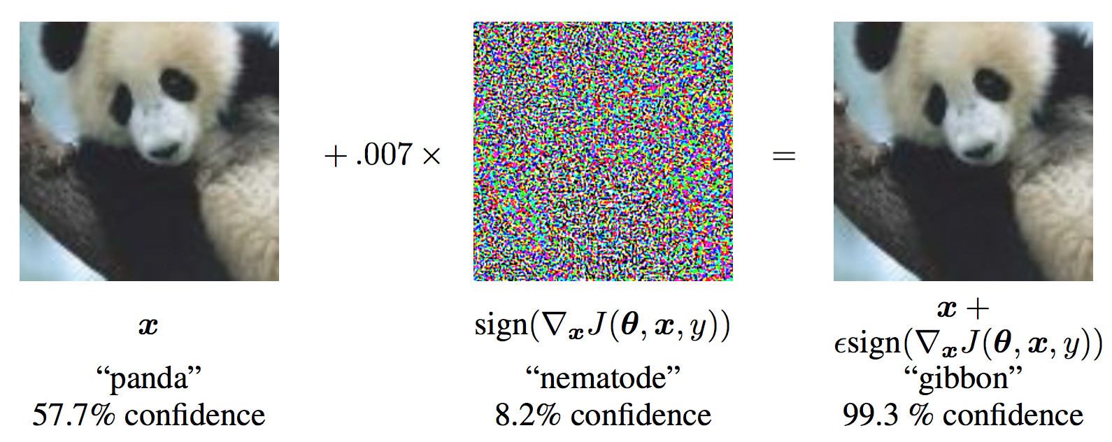
需要注意的是，A——>B，其中A为实际值，B为预测值。随着模型扰动量的增加，预测值也越来越离谱。与此同时，随着扰动量的增加，我们可以看到模型也变得越来越模糊。由于本实验是对黑白图片数字进行识别，其所具有的特征点（即维度）相对比较少，因此想要使模型预测错误率很高，扰动量也必须加到很大。如果是复杂度较高的图片，只需要增加一点扰动量便可以，使错误率增加的很大。例如，经典熊猫图，由于其图片复杂度较高，因此只需要添加0.007的扰动量，便可以使预测错误率达到99.3%。

fgsm_panda_image

小二的安全指北

关注

18
点赞
踩
123

收藏

觉得还不错? 一键收藏
1
评论
FGSM对抗样本算法实现

最著名的对抗样本算法应该就是Fast Gradient Sign Attack（FGSM）快速梯度算法，其原理是，在白盒环境下，通过求出模型对输入数据的导数，用函数求得其梯度方向，再乘以步长，得到的就是其扰动量，将这个扰动量加在原来的输入上，就得到了在FGSM攻击下的样本，这个样本很大概率上可以使模型分类错误，这样就达到了攻击的目的。我们令原始的输入为x，输出为y。则FGSM的攻击表达式为：（1）由公式1可知，FGSM实质上就是一...
复制链接

扫一扫