【多模态】BLIP模型技术学习

前言

最近多模态模型特别火，从头开始学习！在前面写的几篇里面学习了MiniCPM-V、ViT和CLIP之后，今天学习一下BLIP模型，记录学习过程，主要是模型架构、训练方式和相关源代码。欢迎批评指正，一起学习~~

1. 统一的视觉-语言理解和生成的预训练

• BLIP出自OpenAI发表在ICML 2022的论文BLIP: Bootstrapping Language-Image Pre-training for Unified Vision-Language Understanding and Generation
• 提出了一个简单但强大的框架MED，使用自监督学习和对比学习等技术实现视觉和语言的联合预训练，模型能够同时处理理解和生成任务
• 提出了一种对爬取的噪音数据进行过滤清洗的方法CapFilt
  

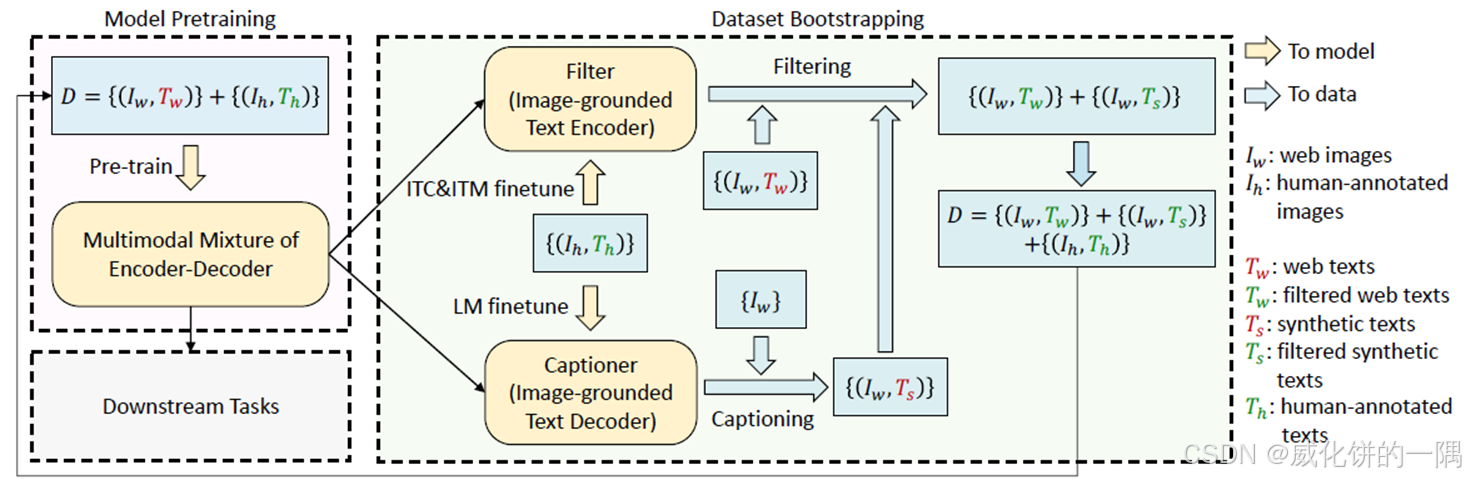
2. 预训练模型架构

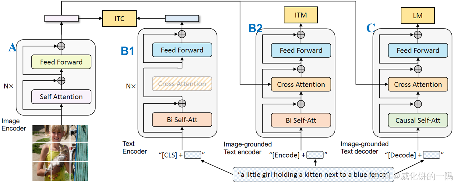
编码器-解码器MED(Multimodal mixture of Encoder-Decoder)

• 图片编码器A：ViT
• 编码器B1/B2：bert的encoder，B1是B2的一部分，计算ITC单文本编码时跳过cross attention层
• 解码器C：bert的decoder，和编码器B共享cross attention和feed forward层参数
  

架构上，找到pretrain的代码，在BLIP_Pretrain的init部分可以看到BLIP使用的编码器和解码器并且encoder和decoder通过对象引用的方式共享参数

# ViT
msg = self.visual_encoder.load_state_dict(state_dict, strict=False)

# 编码器，bert的encoder，代码中叫text_encoder
encoder_config = BertConfig.from_json_file(med_config)
encoder_config.encoder_width = vision_width
self.text_encoder = BertModel.from_pretrained('bert-base-uncased', config=encoder_config, add_pooling_layer=False)
self.text_encoder.resize_token_embeddings(len(self.tokenizer))
text_width = self.text_encoder.config.hidden_size

# create the decoder, bert的BertLMHeadModel，代码中叫text_decoder
decoder_config = BertConfig.from_json_file(med_config)
decoder_config.encoder_width = vision_width
self.text_decoder = BertLMHeadModel.from_pretrained('bert-base-uncased', config=decoder_config)
self.text_decoder.resize_token_embeddings(len(self.tokenizer))

# 除了一开始的self-attention层，encoder和decoder共享参数
tie_encoder_decoder_weights(self.text_encoder, self.text_decoder.bert, '', '/attention')

3.BLIP的预训练Loss

预训练包含3个loss的计算，分别是：

• Image-Text Contrastive Loss (ITC) – 图文对比学习，在隐空间对齐图片编码器和文本编码器的输出
• Image-Text Matching Loss (ITM) - 二分类任务，让模型判断图文是否一致
• Language Modeling Loss (LM) – 下一词预测，让模型学会给定图片输出caption

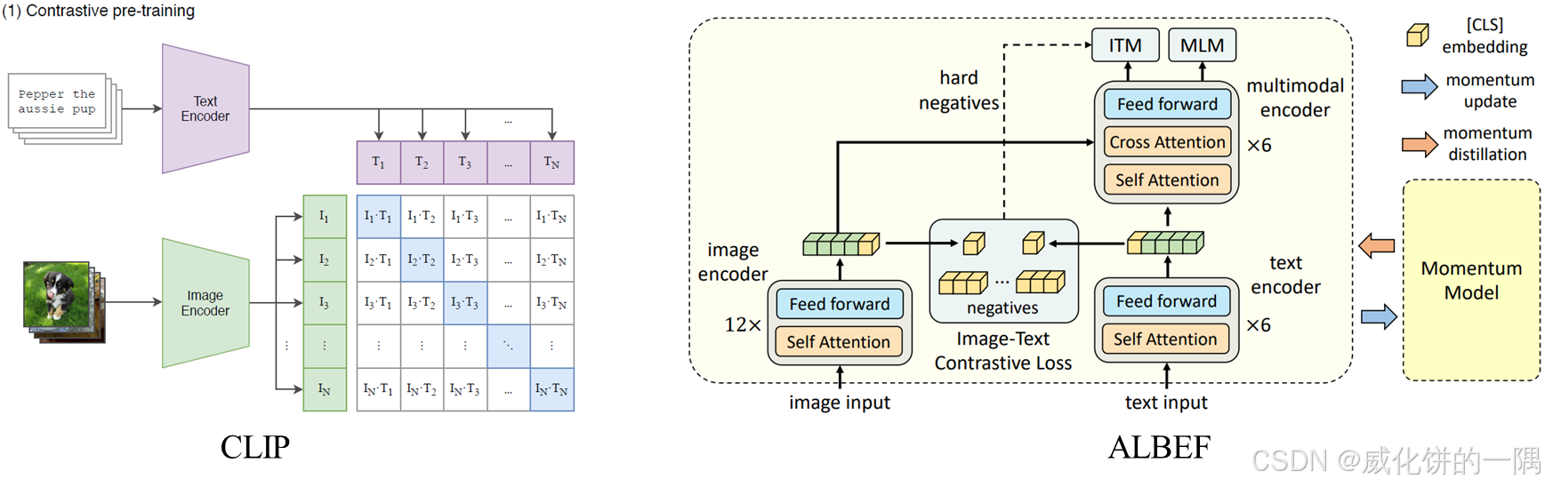
3.1图文对比学习ITC

• [与CLIP区别] 左图为CLIP，右图为使用了一个teacher model输出软的标签，和CLIP的区别在于，计算loss时，用了来自一个momentum model的软标签而不是0-1标签，ALBEF中提到在训练数据中有噪音时，这样计算会更稳定
  

• [Momentum model架构] 这个Momentum model只包含encoder部分不包含decoder，架构和编码器B1/B2一样，会用于ITC损失计算。在建立momentum的时候，还创建了队列，用于存储图-文对信息，在对比学习计算时，输入的一个batch的image会和这个长的队列里面所有的文本计算相似度

# create momentum encoders
self.visual_encoder_m, vision_width = create_vit(vit, image_size)
self.vision_proj_m = nn.Linear(vision_width, embed_dim)
self.text_encoder_m = BertModel(config=encoder_config, add_pooling_layer=False)
self.text_proj_m = nn.Linear(text_width, embed_dim)

self.model_pairs = [
    [self.visual_encoder, self.visual_encoder_m],
    [self.vision_proj, self.vision_proj_m],
    [self.text_encoder, self.text_encoder_m],
    [self.text_proj, self.text_proj_m]
]
self.copy_params()

# create the queue
self.register_buffer("image_queue", torch.randn(embed_dim, queue_size))
self.register_buffer("text_queue", torch.randn(embed_dim, queue_size))
self.register_buffer("queue_ptr", torch.zeros(1, dtype=torch.long))

3.1.1 图文对比学习loss计算包括2个步骤

• 【步骤1：momentum model特征计算】图和文本分别经过各自编码器投影到隐空间，把当前数据和队列里面之前数据拼接，扩大样本量，算出来sim_i2t_targets和sim_t2i_targets，作为ITC计算时的标签(这里面的相似度矩阵sim_i2t_m、sim_t2i_m不一定是方阵)

# get momentum features
with torch.no_grad():
    self._momentum_update()  # teacher model update with running average
    image_embeds_m = self.visual_encoder_m(image)
    image_feat_m = F.normalize(self.vision_proj_m(image_embeds_m[:, 0, :]), dim=-1)
    image_feat_all = torch.cat([image_feat_m.t(), self.image_queue.clone().detach()], dim=1)

    text_output_m = self.text_encoder_m(
        text.input_ids,
        attention_mask=text.attention_mask,
        return_dict=True,
        mode='text'
    )
    text_feat_m = F.normalize(self.text_proj_m(text_output_m.last_hidden_state[:, 0, :]), dim=-1)
    text_feat_all = torch.cat([text_feat_m.t(), self.text_queue.clone().detach()], dim=1)  # 转置了
    sim_i2t_m = image_feat_m @ text_feat_all / self.temp  # sim_i2t_m的形状为(batch_size, queue_size)
    sim_t2i_m = text_feat_m @ image_feat_all / self.temp

    sim_targets = torch.zeros(sim_i2t_m.size()).to(image.device)
    sim_targets.fill_diagonal_(1)  # 主对角线为1
    # 用momentum的软标签平滑
    sim_i2t_targets = alpha * F.softmax(sim_i2t_m, dim=1) + (1 - alpha) * sim_targets
    sim_t2i_targets = alpha * F.softmax(sim_t2i_m, dim=1) + (1 - alpha) * sim_targets

• 【步骤2：KL散度的loss计算】分别算图-文相似度的loss和文-图相似度的loss，类似知识蒸馏，实际上算的是KL散度

sim_i2t = image_feat @ text_feat_all / self.temp  # (batch_size, queue_size)
sim_t2i = text_feat @ image_feat_all / self.temp

# 每一行是第i张图和文本的相似度，行上进行softmax
# 逐元素相乘，每行计算sum，均值作为loss (可以看成每行的对数概率分布与对应行的目标分布逐元素相乘)
loss_i2t = -torch.sum(F.log_softmax(sim_i2t, dim=1) * sim_i2t_targets, dim=1).mean()
loss_t2i = -torch.sum(F.log_softmax(sim_t2i, dim=1) * sim_t2i_targets, dim=1).mean()

loss_ita = (loss_i2t + loss_t2i) / 2

self._dequeue_and_enqueue(image_feat_m, text_feat_m)

3.1.2 KL散度/交叉熵的理解

  CLIP是计算的交叉熵，而BLIP是类似知识蒸馏的方式计算KL散度（P为目标标签分布，Q为预测分布）
熵
$$H(P)=-\sum _{x}P(x)logP(x)$$
交叉熵
$$H(P,Q)=-\sum _{x}P(x)logQ(x)$$
KL散度/相对熵
$$D_{KL}(P||Q)=\sum _{x}P(x)log\frac{P(x)}{Q(x)}$$

  对于一个满足分布$P(x)$的随机变量$x$，最优编码下的平均长度为熵$H(P)$。但是如果搞错了，以为随机变量分布是$Q(x)$，用$Q(x)$来编码，最佳长度为$H(P,Q)=-{\sum }_{x}P(x)logQ(x)$，多出来的这部分就是KL散度（相对熵）$D_{KL}(P||Q)=H(P,Q)-H(P)$。
  此外，KL散度可以展开为$D_{KL}(P||Q)={\sum }_{x}P(x)logP(x)-{\sum }_{x}P(x)logQ(x)$。由于由于$P(x)$是已知的真实标签分布，所以$H(P)$是一个常数项，所以ITC的loss优化时，和代码中呈现的那样，要最小化KL散度，实际上是在最小化交叉熵$H(P,Q)$。

3.2 图文匹配ITM

  计算图文匹配损失时，是一个二分类任务，即图和文是否匹配，所以首先要抽取负样本，代码中呈现为

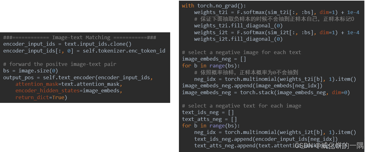
  接着构建图-文的负样本对，图和文正好反过来，计算二分类损失

text_ids_neg = torch.stack(text_ids_neg, dim=0)
text_atts_neg = torch.stack(text_atts_neg, dim=0)

text_ids_all = torch.cat([encoder_input_ids, text_ids_neg], dim=0)
text_atts_all = torch.cat([text.attention_mask, text_atts_neg], dim=0)

# 和上面对比，image_embeds_all和text_ids_all是不匹配的，反过来一正一负对应
image_embeds_all = torch.cat([image_embeds_neg, image_embeds], dim=0)
image_atts_all = torch.cat([image_atts, image_atts], dim=0)

output_neg = self.text_encoder(
    text_ids_all,
    attention_mask=text_atts_all,
    encoder_hidden_states=image_embeds_all,
    encoder_attention_mask=image_atts_all,
    return_dict=True,
)

vl_embeddings = torch.cat([output_pos.last_hidden_state[:, 0, :], output_neg.last_hidden_state[:, 0, :]], dim=0)
vl_output = self.itm_head(vl_embeddings)

itm_labels = torch.cat([
    torch.ones(bs, dtype=torch.long),
    torch.zeros(2 * bs, dtype=torch.long)
], dim=0).to(image.device)
loss_itm = F.cross_entropy(vl_output, itm_labels)

图文匹配涉及的crossattention

• 值得注意的是，图文匹配时，里面文本先经过一个标准的self-attention模块，然后有一个图-文输入的cross-attention模块
• encoder_input_ids是文本输入，形状为[batch_size,seq_len,text_emb_dim]
• attention_mask是0-1文本掩码，用于指示哪部分进行了padding，形状为[batch_size,seq_len]
• 图片部分和文本类似，区别是图片的掩码image_atts是全1

output_pos = self.text_encoder(
    encoder_input_ids,
    attention_mask=text.attention_mask,
    encoder_hidden_states=image_embeds,
    encoder_attention_mask=image_atts,
    return_dict=True,
)

Image-grounded text_encoder数据流
1. 在text_encoder中，具体到每一个bertlayer，首先文本部分先过一个self_attention层，取[CLS]的输出

self_attention_outputs = self.attention(
    hidden_states,    attention_mask,    head_mask,
    output_attentions=output_attentions
)
attention_output = self_attention_outputs[0]

2. 然后是交叉注意力层，文本的[CLS]作为query，图像特征作为key和value，运算之后取[0]输出

cross_attention_outputs = self.crossattention(
    attention_output,    attention_mask,
    head_mask,
    encoder_hidden_states,    encoder_attention_mask,
    output_attentions=output_attentions
)
attention_output = cross_attention_outputs[0]

** 其实交叉注意力层就是普通的self-attention层，只不过Wk和Wv矩阵的形状要和图片特征适配

if is_cross_attention:
    self.key = nn.Linear(config.encoder_width, self.all_head_size)
    self.value = nn.Linear(config.encoder_width, self.all_head_size)

if is_cross_attention:
    key_layer = self.transpose_for_scores(self.key(encoder_hidden_states))
    value_layer = self.transpose_for_scores(self.value(encoder_hidden_states))

3.3 LM下一词预测loss

第三个loss是下一词预测loss，具体计算为：

• 文本第一个词为<bos>，输入到text_decoder的包含文本和图像，预期要模型学会完美输出label
• decoder_targets 中把文本padding的id替换为-100，这样在计算交叉熵时会忽略padding的部分
• decoder的下一词预测这里，架构图里面有一个causal self-attention（预测下一个词时，只能看到前面的词，看不到下一个词以及之后的词语），由mask机制实现

**在encoder部分提到的Bi self-attention就是基础的自注意力模块（本来就是双向的，计算所有文本的q和k的相似度，不会只计算前面或者后面的

##================= LM ========================##
decoder_input_ids = text.input_ids.clone()
decoder_input_ids[:, 0] = self.tokenizer.bos_token_id
decoder_targets = decoder_input_ids.masked_fill(decoder_input_ids == self.tokenizer.pad_token_id, -100)

decoder_output = self.text_decoder(
    decoder_input_ids,
    attention_mask=text.attention_mask,
    encoder_hidden_states=image_embeds,
    encoder_attention_mask=image_atts,
    labels=decoder_targets,
    return_dict=True,
)

loss_lm = decoder_output.loss

BLIP的LM的loss计算有2个点需要注意：mask的计算和最后LM的运算形式

3.3.1 mask计算

• 首先，如果是普通的padding的mask，在self-attention计算前，会把取值为{0,1}的文本mask，变成取值为{0,-10000}

extended_attention_mask = extended_attention_mask.to(dtype=self.dtype)  # fp16 compatibility
extended_attention_mask = (1.0 - extended_attention_mask) * -10000.0

• 接着在计算attention分数时，是对softmax之前原始的注意力分数加上这个mask，而不是取数值乘以{0,1}的mask

# Take the dot product between "query" and "key" to get the raw attention scores.
attention_scores = torch.matmul(query_layer, key_layer.transpose(-1, -2))
attention_scores = attention_scores / math.sqrt(self.attention_head_size)

if attention_mask is not None:
    # Apply the attention mask is (precomputed for all layers in BertModel forward() function)
    attention_scores = attention_scores + attention_mask

# Normalize the attention scores to probabilities.
attention_probs = nn.Softmax(dim=-1)(attention_scores)

# This is actually dropping out entire tokens to attend to, which might
# seem a bit unusual, but is taken from the original Transformer paper.
attention_probs_dropped = self.dropout(attention_probs)
context_layer = torch.matmul(attention_probs_dropped, value_layer)

• 在反向传播过程中，使用0进行掩码会导致梯度为0，这意味着模型无法学习这些位置的信息，而使用较大的负数，虽然实际上这些位置的权重接近于0，但它们仍然可以传递梯度

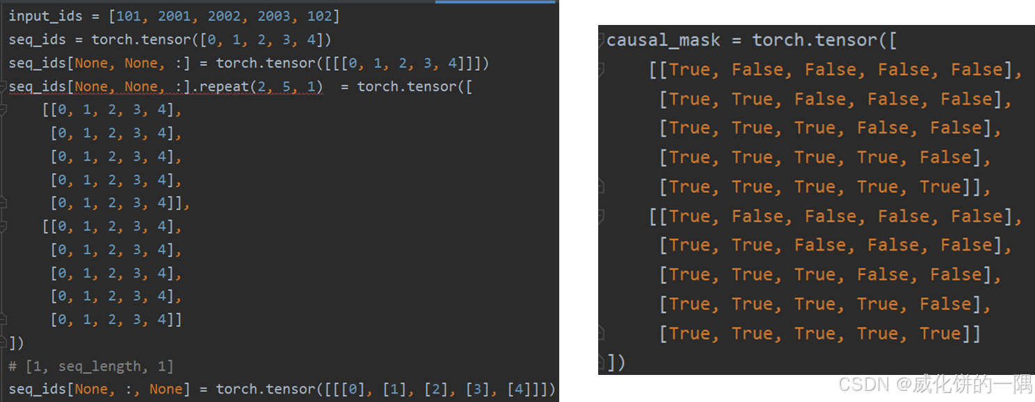
Causal Mask
  下一词预测时的mask叫causal mask，具体生成方式结合代码更容易理解，就是不想让时间步为t的看到时间步为t+1的数据

batch_size, seq_length = input_shape
seq_ids = torch.arange(seq_length, device=device)
causal_mask = seq_ids[None, None, :].repeat(batch_size, seq_length, 1) <= seq_ids[None, :, None]
extended_attention_mask = causal_mask[:, None, :, :] * attention_mask[:, None, None, :]

  上面的最后一行代码有一些抽象，可以从例子里面看明白，其中[None,None,:]和[None, :, None]是进行了升维

3.3.2 LM的loss计算形式

• 最后LM的loss计算时，还有一个shift的操作
• prediction_scores 的形状为[batch_size,seq_len,vocab_size]
• labels=decoder_targets，形状为[batch_size,seq_len]，其中labels[:,0]是<bos>
• prediction_scores和labels都移动了一位，形状正好match
• 训练阶段是有完整的label作为query输入的，完美的情况下bert并行的一次推理把label都推理出来。之后训练晚的推理阶段，输入的文本query只有prompt+<bos>，要一个个词解码

outputs = self.bert(
    input_ids,
    attention_mask=attention_mask,
    inputs_embeds=inputs_embeds,
    encoder_hidden_states=encoder_hidden_states,
    encoder_attention_mask=encoder_attention_mask,
)
sequence_output = outputs[0]
prediction_scores = self.cls(sequence_output)

if labels is not None:
    # we are doing next-token prediction; shift prediction scores and input ids by one
    shifted_prediction_scores = prediction_scores[:, :-1, :].contiguous()
    labels = labels[:, 1:].contiguous()
    loss_fct = CrossEntropyLoss(reduction=reduction, label_smoothing=0.1)
    lm_loss = loss_fct(shifted_prediction_scores.view(-1, self.config.vocab_size), labels.view(-1))

参考链接

1. BLIP官方的blog解读：https://blog.salesforceairesearch.com/blip-bootstrapping-language-image-pretraining/
2. BLIP的ICML的论文、视频和ppt链接：https://icml.cc/virtual/2022/spotlight/16016