一阶低通滤波器和巴特沃斯滤波器效果对比

一阶低通滤波器和巴特沃斯滤波器效果对比

效果对比

下是python程序，直接复制过去运行使用。

import numpy as np
import matplotlib.pyplot as plt
from scipy.signal import butter, filtfilt
import matplotlib.font_manager as fm
from matplotlib.widgets import Slider


# 一阶低通滤波器
def low_pass_filter(x, alpha, y_prev=0):
    y = alpha * x + (1 - alpha) * y_prev
    return y


# 一阶巴特沃斯滤波器
def butter_lowpass_filter(data, cutoff, fs, order=1):
    nyq = 0.5 * fs
    normal_cutoff = cutoff / nyq
    b, a = butter(order, normal_cutoff, btype='low', analog=False)
    y = filtfilt(b, a, data)
    return y


# 生成不规则的原始信号
t = np.linspace(0, 10, 1000)  # 时间向量
steps = np.random.randn(len(t))  # 随机步长
x = np.cumsum(steps)  # 随机游走
noise = 0.5 * np.sin(2 * np.pi * 50 * t) + 0.5 * np.random.normal(size=len(t))  # 高频噪声
x_noisy = x + noise  # 带高频噪声的原始信号

# 叠加正弦波
sin_amplitude = 10  # 初始正弦波幅度
sin_wave = sin_amplitude * np.sin(2 * np.pi * 1 * t)  # 1 Hz 正弦波
x_noisy_with_sin = x_noisy + sin_wave  # 带正弦波的原始信号

# 滤波器参数
fs = 100  # 采样频率 (Hz)
cutoff = 2  # 初始截止频率 (Hz)
alpha = 0.1  # 初始滤波系数
order = 1  # 初始滤波器阶数

# 设置中文字体
font_prop = fm.FontProperties(family='SimHei')  # 使用系统自带的 SimHei 字体
plt.rcParams['font.sans-serif'] = ['SimHei']  # 设置全局字体
plt.rcParams['axes.unicode_minus'] = False  # 正常显示负号

# 初始化滤波器响应
y_low_pass = [low_pass_filter(x_noisy_with_sin[0], alpha)]
for i in range(1, len(x_noisy_with_sin)):
    y_low_pass.append(low_pass_filter(x_noisy_with_sin[i], alpha, y_low_pass[-1]))

y_low_pass = np.array(y_low_pass)
y_butter = butter_lowpass_filter(x_noisy_with_sin, cutoff, fs, order)

# 计算一阶导数
y_low_pass_derivative = np.gradient(y_low_pass, t[1] - t[0])
y_butter_derivative = np.gradient(y_butter, t[1] - t[0])

# 创建图形
fig, axs = plt.subplots(2, 1, figsize=(12, 8))

# 绘制初始图像
line1, = axs[0].plot(t, x_noisy_with_sin, label='带噪声和正弦波的原始信号', color='gray', alpha=0.7)
line2, = axs[0].plot(t, y_low_pass, label='一阶低通滤波器', linewidth=2)
line3, = axs[0].plot(t, y_butter, label='一阶巴特沃斯滤波器', linewidth=2, linestyle='--')
axs[0].set_xlabel('时间 (s)', fontproperties=font_prop)
axs[0].set_ylabel('幅度', fontproperties=font_prop)
axs[0].legend(prop=font_prop)
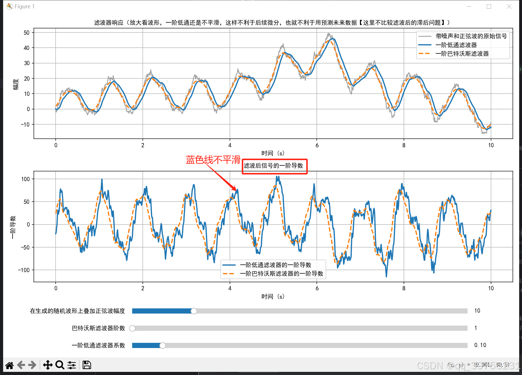
axs[0].set_title('滤波器响应（放大看波形，一阶低通还是不平滑，这样不利于后续微分，也就不利于用预测未来数据【这里不比较滤波后的滞后问题】）', fontproperties=font_prop)
axs[0].grid(True)

line4, = axs[1].plot(t, y_low_pass_derivative, label='一阶低通滤波器的一阶导数', linewidth=2)
line5, = axs[1].plot(t, y_butter_derivative, label='一阶巴特沃斯滤波器的一阶导数', linewidth=2, linestyle='--')
axs[1].set_xlabel('时间 (s)', fontproperties=font_prop)
axs[1].set_ylabel('一阶导数', fontproperties=font_prop)
axs[1].legend(prop=font_prop)
axs[1].set_title('滤波后信号的一阶导数', fontproperties=font_prop)
axs[1].grid(True)

# 创建滑动条
ax_alpha = fig.add_axes([0.25, 0.02, 0.65, 0.03])
ax_order = fig.add_axes([0.25, 0.07, 0.65, 0.03])
ax_amplitude = fig.add_axes([0.25, 0.12, 0.65, 0.03])

slider_alpha = Slider(ax=ax_alpha, label='一阶低通滤波器系数', valmin=0.01, valmax=1, valinit=alpha)
slider_order = Slider(ax=ax_order, label='巴特沃斯滤波器阶数', valmin=1, valmax=5, valinit=order, valstep=1)
slider_amplitude = Slider(ax=ax_amplitude, label='在生成的随机波形上叠加正弦波幅度', valmin=1, valmax=50, valinit=sin_amplitude)


# 更新函数
def update(val):
    global y_low_pass, y_butter, y_low_pass_derivative, y_butter_derivative, x_noisy_with_sin
    alpha = slider_alpha.val
    order = int(slider_order.val)
    sin_amplitude = slider_amplitude.val

    # 重新生成带正弦波的原始信号
    sin_wave = sin_amplitude * np.sin(2 * np.pi * 1 * t)
    x_noisy_with_sin = x_noisy + sin_wave

    # 重新计算滤波器响应
    y_low_pass = [low_pass_filter(x_noisy_with_sin[0], alpha)]
    for i in range(1, len(x_noisy_with_sin)):
        y_low_pass.append(low_pass_filter(x_noisy_with_sin[i], alpha, y_low_pass[-1]))

    y_low_pass = np.array(y_low_pass)
    y_butter = butter_lowpass_filter(x_noisy_with_sin, cutoff, fs, order)

    # 重新计算一阶导数
    y_low_pass_derivative = np.gradient(y_low_pass, t[1] - t[0])
    y_butter_derivative = np.gradient(y_butter, t[1] - t[0])

    # 更新图像
    line1.set_ydata(x_noisy_with_sin)
    line2.set_ydata(y_low_pass)
    line3.set_ydata(y_butter)
    line4.set_ydata(y_low_pass_derivative)
    line5.set_ydata(y_butter_derivative)

    fig.canvas.draw_idle()


# 绑定滑动条事件
slider_alpha.on_changed(update)
slider_order.on_changed(update)
slider_amplitude.on_changed(update)

plt.tight_layout(rect=[0, 0.15, 1, 1])
plt.show()

结论：

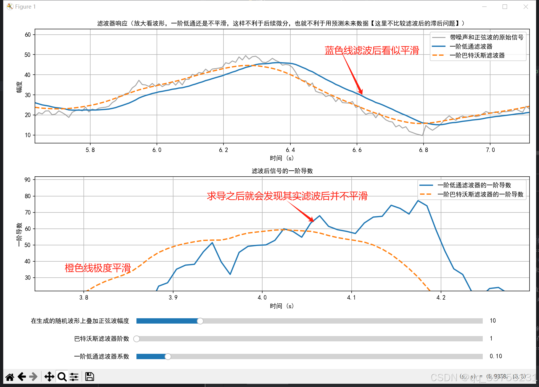
巴特沃斯滤波器非常平滑导数也是平滑，这样有利于后续用泰勒展开的方法来预测未来点。
一阶低通滤波器就算滤波效果调高了放大了看也是不平滑的，一阶导数更是没法看。这种状态很难使用泰勒展开方法预测未来点。