【yolov8s-pose三种模型推理时间以及不同batch下GPU利用率对比（附代码）

yolov8s-pose三种模型推理时间以及不同batch下GPU利用率对比（附代码）

具体测试数据和代码：测试数据和代码
3060显卡测试，其他显卡可自行测试
模型的输入都是640x640,不同batch进行的推理情况，每个batch测试10次，三种模型在验证集上的预测精度相同
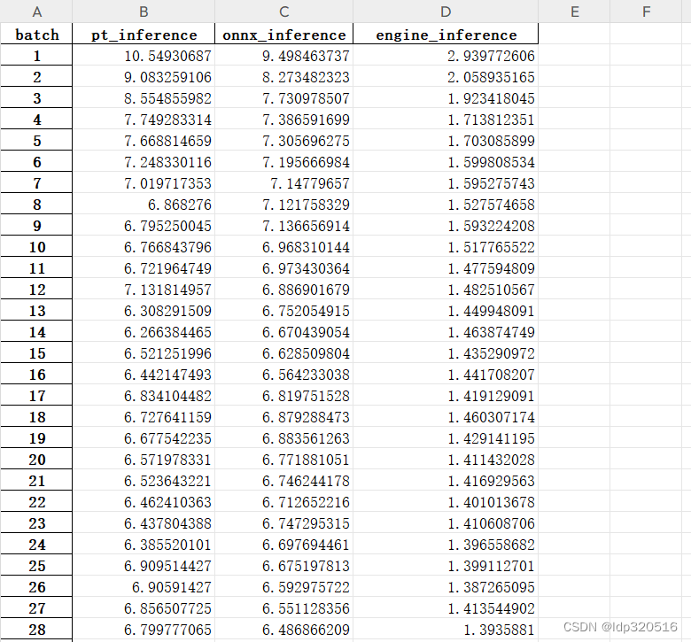三种模型不同batch下的前向推理时间

pt模型和onnx模型使用float32推理，engine使用fp16推理
onnx模型动态batch，动态宽高，使得模型的复杂度变高，造成以下onnx模型性能的降低
Tensorrt模型不能动态宽高，动态宽高会造成模型的复杂度变高，性能反而降低，只使用动态batch
1、模型推理速度(inference：10轮里面的平均时间)

engine模型前向推理速度基本都在单张图平均2ms以下，最低的时候时为batch_size设置为58时
2、preprocess+inference+postprocess（10轮里面的平均时间）

engine模型处理每张图片的平均时间
3、显存（10轮里面最大的显存）


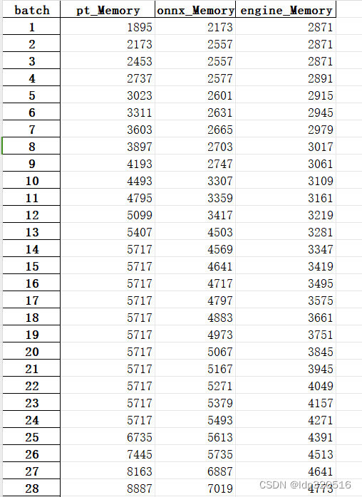
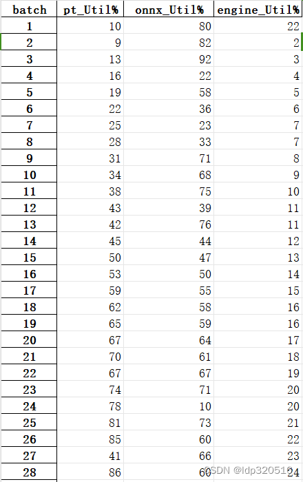
随之batch_size的增加，显存随着增加，batch_size设置为61的时候，显存降低，但是下面的GPU利用率达到最高，当batch_size达到56的时候，onnx显存撑爆
4、GPU利用率（10轮里面最大的利用率）

# import pandas as pd
# # 读取txt文件
# data = pd.read_csv('gpuinfo_engine.txt', delimiter=' ')
#
# # 按照第一列（'batch'列）进行分组，并计算每组的平均值
# grouped = data.groupby('batch')
# average_values = grouped.max()
#
# # 将计算结果存储到新的DataFrame对象中
# result = pd.DataFrame(average_values)
# result.to_excel('gpuinfo_engine.xlsx', index=True)

import pandas as pd
import matplotlib.pyplot as plt

# 读取Excel表格
df = pd.read_excel('memory.xlsx')

# 绘制图形，使用不同颜色表示三列数据
plt.plot(df['batch'], df['pt_Memory'], color='red', label='pt_Memory')
plt.plot(df['batch'], df['onnx_Memory'], color='blue', label='onnx_Memory')
plt.plot(df['batch'], df['engine_Memory'], color='green', label='engine_Memory')

# 找到每条线的最低点
min_col2 = df['pt_Memory'].min()
min_index_col2 = df['pt_Memory'].idxmin()

min_col3 = df['onnx_Memory'].min()
min_index_col3 = df['onnx_Memory'].idxmin()

min_col4 = df['engine_Memory'].min()
min_index_col4 = df['engine_Memory'].idxmin()


# 在最低点处添加注释
plt.scatter(df['batch'][min_index_col2], min_col2, color='black')
plt.scatter(df['batch'][min_index_col3], min_col3, color='black')
plt.scatter(df['batch'][min_index_col4], min_col4, color='black')

x1 = df['batch'][min_index_col2]
y1 = min_col2

x2 = df['batch'][min_index_col3]
y2 = min_col3

x3 = df['batch'][min_index_col4]
y3 = min_col4

for x, y in zip([x1], [y1]):
    plt.annotate('(%d, %d)' % (x, y), xy=(x, y), xytext=(0, 10), textcoords='offset points')
for x, y in zip([x2], [y2]):
    plt.annotate('(%d, %d)' % (x, y), xy=(x, y), xytext=(0, 10), textcoords='offset points')
for x, y in zip([x3], [y3]):
    plt.annotate('(%d, %d)' % (x, y), xy=(x, y), xytext=(0, 10), textcoords='offset points')

plt.xlabel('batch')
plt.ylabel('GPU Memory /MB')
plt.title('GPU Memory of three model')
plt.legend()
plt.savefig('memory.png')
plt.show()

# # 创建子图
# fig, ax = plt.subplots()
#
# # 绘制col1和col2列的折线图
# ax.plot(df['batch'], df['Memory'], label='Memory',color='blue')
# ax.set_xlabel('batch')
# ax.set_ylabel('Memory')
# ax.legend()
#
# # 绘制col1和col3列的折线图
# ax2 = ax.twinx()
# ax2.plot(df['batch'], df['Util'], label='Util',color='green')
# ax2.set_ylabel('Util')
# ax2.legend()

# plt.plot(df['batch'], df['Memory'], color='blue', label='pt_Memory')
# plt.plot(df['batch'], df['Util'], color='green', label='pt_Util')

# plt.xlabel('batch')
# plt.ylabel('ms')
# plt.title('Plot of three columns')

# # 找到每条线的最低点
# min_col2 = df['Memory'].min()
# min_index_col2 = df['Memory'].idxmin()
#
# min_col3 = df['Util'].min()
# min_index_col3 = df['Util'].idxmin()
#
#
# # 在最低点处添加注释
# plt.scatter(df['batch'][min_index_col2], min_col2, color='green')
# plt.scatter(df['batch'][min_index_col3], min_col3, color='blue')
# x1 = df['batch'][min_index_col2]
# y1 = min_col2
#
# x2 = df['batch'][min_index_col3]
# y2 = min_col3
#
# for x, y in zip([x1], [y1]):
#     plt.annotate('(%d, %d)' % (x, y), xy=(x, y), xytext=(0, 10), textcoords='offset points')
# for x, y in zip([x2], [y2]):
#     plt.annotate('(%d, %d)' % (x, y), xy=(x, y), xytext=(0, 10), textcoords='offset points')
#
# plt.legend()
# plt.show()