Code | 线性分类器：批量感知算法+Ho_Kashyap算法（二分类）+MSE多类扩展

1. 数据

2.

import matplotlib.pyplot as plt
import numpy as np

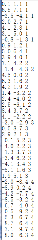
x = np.loadtxt('data.txt')
b = np.ones(40)
y = np.insert(x, 0, b, 1)  # 增广

class BatchPerception():
    def __init__(self, w1, w2, y):
        self.w1 = w1
        self.w2 = w2
        self.a = np.zeros(3)
        self.count = 0
        self.lr = 1
        self.y = y

    def preprocess(self):
        y_temp = self.y.copy()
        y_w1 = y_temp[(self.w1 - 1) * 10:self.w1 * 10, 0:3]
        y_w2 = -1 * y_temp[(self.w2 - 1) * 10:self.w2 * 10, 0:3] # 规范化
        y_w = np.concatenate((y_w1, y_w2), axis=0)
        return y_w

    def train(self):
        y_w = self.preprocess()
        for j in range(1000):
            Y = []

            for i in range(20):
                if np.inner(self.a, y_w[i]) <= 0:
                    Y.append(y_w[i])
#                    print(np.inner(self.a, y[i][0:3]))
            if len(Y) == 0:
                print(self.w1, '和', self.w2, self.a, self.count)
                break
            Y_sum = np.sum(Y, axis=0)
            self.a = self.a + self.lr * Y_sum
            self.count += 1

    def visualization(self):
        y_temp = self.y.copy()
        # y_temp[10:20] = -1 * y_temp[10:20]
        # y_temp[30:40] = -1 * y_temp[30:40]
        y_w1 = y_temp[(self.w1 - 1) * 10:self.w1 * 10, 0:3]
        y_w2 = y_temp[(self.w2 - 1) * 10:self.w2 * 10, 0:3]
        y = np.concatenate((y_w1, y_w2), axis=0)
        ax = plt.gca()
        plt.scatter(y[0:10, 1], y[0:10, 2], s=16, label='sample of w' + str(self.w1))
        plt.scatter(y[10:20, 1], y[10:20, 2], s=16, label='sample of w' + str(self.w2))
        x_min = np.min(y[:, 1])
        x_max = np.max(y[:, 1])
        x_plot = np.arange(x_min, x_max, (x_max - x_min) / 100)
        y_plot = -(self.a[1] * x_plot + self.a[0]) / self.a[2]
        plt.plot(x_plot, y_plot, linewidth=2, label='boundary')
        plt.legend()
        plt.title('classification result by BatchPerception between w' + str(self.w1) + ' and w' + str(self.w2))
        ax.set_xlabel('x1')
        ax.set_ylabel('x2')
        plt.savefig('BP'+str(self.w1)+str(self.w2)+'.png')
        plt.show()


class Ho_Kashyap():
    def __init__(self, w1, w2, y):
        self.w1 = w1
        self.w2 = w2
        self.y = y
        self.count = 0
        self.a = np.zeros(3)
        self.b = 1*np.ones(20)
        self.lr = 0.5

    def preprocess(self):
        y_temp = self.y.copy()
        y_w1 = y_temp[(self.w1 - 1) * 10:self.w1 * 10, 0:3]
        y_w2 = -1 * y_temp[(self.w2 - 1) * 10:self.w2 * 10, 0:3] # 规范化
        y_w = np.concatenate((y_w1, y_w2), axis=0)
        return y_w

    def train(self):
        y = self.preprocess()
        for i in range(1000):
            e = np.subtract(np.matmul(y, self.a), self.b)
            e_ = 0.5*(e+np.absolute(e))
            self.b = self.b + 2*self.lr*e_
            self.a = np.matmul(np.linalg.pinv(y), self.b)
        print(np.linalg.norm(e))
        # print(self.a, self.b)

    def visualization(self):
        y_temp = self.y.copy()
        y_w1 = y_temp[(self.w1 - 1) * 10:self.w1 * 10, 0:3]
        y_w2 = y_temp[(self.w2 - 1) * 10:self.w2 * 10, 0:3]
        y = np.concatenate((y_w1, y_w2), axis=0)
        ax = plt.gca()
        plt.scatter(y[0:10, 1], y[0:10, 2], s=16, label='sample of w' + str(self.w1))
        plt.scatter(y[10:20, 1], y[10:20, 2], s=16, label='sample of w' + str(self.w2))
        x_min = np.min(y[:, 1])
        x_max = np.max(y[:, 1])
        x_plot = np.arange(x_min, x_max, (x_max - x_min) / 100)
        y_plot = -(self.a[1] * x_plot + self.a[0]) / self.a[2]
        plt.plot(x_plot, y_plot, linewidth=2, label='boundary')
        plt.legend()
        plt.title('classification result by Ho_Kashyap between w' + str(self.w1) + ' and w' + str(self.w2))
        ax.set_xlabel('x1')
        ax.set_ylabel('x2')
        plt.savefig('HK'+str(self.w1)+str(self.w2)+'.png')
        plt.show()


class MSE_Expand():
    def __init__(self, y):
        self.y = y
        self.a = np.zeros([4, 3]) #4*3 * 3*32
        self.label_train = np.zeros([4, 32])
        self.label_test = np.zeros([4, 8])

    def preprocess(self):
        y_temp = self.y.copy()
        y_train = np.concatenate((y_temp[0:8, 0:3], y_temp[10:18, 0:3], y_temp[20:28, 0:3], y_temp[30:38, 0:3]), axis=0).T  # 3*32
        y_test = np.concatenate((y_temp[8:10, 0:3], y_temp[18:20, 0:3], y_temp[28:30, 0:3], y_temp[38:40, 0:3]), axis=0).T
        for i in range(len(self.label_train)):
            for j in range(len(self.label_train[0])):
                self.label_train[i, j] = int(int(j/8)==i)
        for i in range(len(self.label_test)):
            for j in range(len(self.label_test[0])):
                self.label_test[i, j] = int(int(j/2)==i)
        return y_train, y_test

    def test(self, y_test):
        t = np.arange(1,5)
        test = np.matmul(t, self.label_test)
        result = np.argmax(np.matmul(self.a, y_test), axis=0)+np.ones_like(np.argmax(np.matmul(self.a, y_test), axis=0))
        correct = sum(test == result) / len(self.label_test[0])
        # print(np.matmul(self.a, y_test))
        print(correct)

    def train(self):
        y_train, y_test = self.preprocess()

        a_temp = np.matmul(np.linalg.pinv(y_train.T), self.label_train.T)
        self.a = a_temp.T
        self.test(y_test)



if __name__ == "__main__":
    BP_12 = BatchPerception(1, 2, y)
    BP_23 = BatchPerception(2, 3, y)
    BP_12.train()
    BP_23.train()
    BP_12.visualization()
    BP_23.visualization()

    HP_13 = Ho_Kashyap(1, 3, y)    
    HP_13.train()
    HP_13.visualization()
    HP_24 = Ho_Kashyap(2, 4, y)
    HP_24.train()
    HP_24.visualization()

    ME = MSE_Expand(y)
    ME.train()