


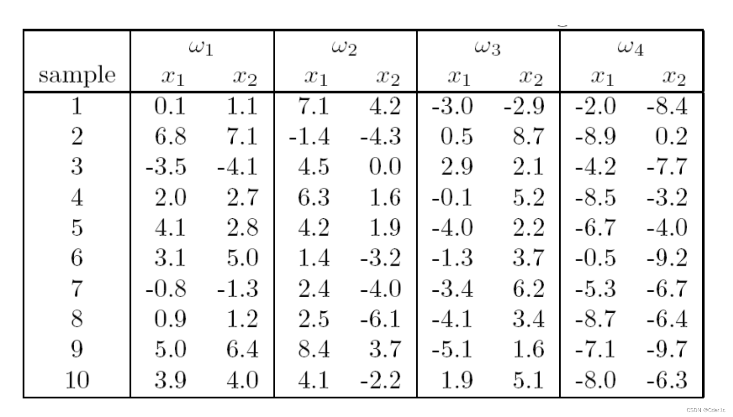
使用数据
Batch Perception算法
原理
设有一组样本
y
1
,
y
2
,
.
.
.
,
y
n
y_1,y_2,...,y_n
y1,y2,...,yn,各样本均规范化表示,我们的目的是找一个解向量
a
a
a ,使
a
T
y
i
>
0
a^T y_i>0
aTyi>0。在线性可分的情况下,满足上式的
a
a
a是无穷的。所以要引出一个损失函数进行优化。这个准则的基本思想是错分样本最少:
J
(
a
)
=
∑
y
∈
Y
(
−
a
T
y
)
J(a)=\sum_{y\in Y}(-a^{T}y)
J(a)=∑y∈Y(−aTy)
Y
Y
Y为错分样本集合。我们采用梯度下降来优化目标函数:
∂
J
∂
a
=
∑
y
∈
Y
(
−
y
)
\frac{\partial J}{\partial a}=\sum_{y\in Y}(-y)
∂a∂J=∑y∈Y(−y)
则有:
a
k
+
1
=
a
k
−
η
∑
y
∈
Y
(
−
y
)
a_{k+1}=a_{k}-η\sum_{y\in Y}(-y)
ak+1=ak−η∑y∈Y(−y)
代码实现
# Define batch perception algorithm
# Input: w1, w2
#   w1: Samples in class 1
#   w2: Samples in class 2
# Output: a, n
#   a: the parameters
#   n: number of iterations
def batch_perception(w1, w2):
    # Generate the normalized augmented samples
    w = trans_sample(w1, w2)

    # Initiation
    a = np.zeros_like(w[1])
    eta = 1                             # Learning rate
    theta = np.zeros_like(w[1])+1e-6    # Termination conditions
    n = 0                               # Number of iterations

    # Implement the algorithm
    while True:
        y = np.zeros_like(w[1])
        for sample in w:
            if np.matmul(a.T, sample) <= 0:
                # the sample is misclassified
                y += sample
        eta_y = eta * y

        if all(np.abs(eta_y)<=theta):
            # if the termination conditions are satisfied, terminate the iteration
            break

        a += eta_y
        n += 1

    print ("The dicision surface a is {}\nThe number of iterations is {}.".format(a, n))
    return a, n
Ho-Kashyap算法
原理
刚才的准则函数都是关注于错分样本,而对正确分类的样本则没有考虑在内。MSE准则函数把求解目标从不等式形式变成了等式形式:求取满足 a T y i = b i a^T y_i=b_i aTyi=bi的权向量。在这里, b i b_i bi是任取的正常数。
如果记矩阵
Y
∈
R
n
∗
d
Y\in R^{n*d}
Y∈Rn∗d且其每行都是一个样本
y
T
y^T
yT,向量
b
=
[
b
1
,
b
2
,
.
.
.
,
b
n
]
T
b=[b_1,b_2,...,b_n]^T
b=[b1,b2,...,bn]T,那么就可以表述为存在
Y
a
=
b
>
0
Ya=b>0
Ya=b>0。为了求解这个问题,使用MSE准则函数:
J
=
∣
∣
Y
a
−
b
∣
∣
2
=
∑
i
=
1
n
(
a
T
y
i
−
b
i
)
2
J=||Ya-b||^2=\sum_{i=1}^{n}(a^T y_i-b_i)^2
J=∣∣Ya−b∣∣2=∑i=1n(aTyi−bi)2
采用梯度下降来优化目标函数:
∂
J
∂
a
=
2
Y
T
(
Y
a
−
b
)
\frac{\partial J}{\partial a}=2Y^T(Ya-b)
∂a∂J=2YT(Ya−b)
∂
J
∂
b
=
−
2
(
Y
a
−
b
)
\frac{\partial J}{\partial b}=-2(Ya-b)
∂b∂J=−2(Ya−b)
则有:
b
k
+
1
=
b
k
+
2
η
k
1
2
(
∂
J
∂
b
−
∣
∂
J
∂
b
∣
)
b_{k+1}=b_k+2η_{k}\frac{1}{2}(\frac{\partial J}{\partial b}-|\frac{\partial J}{\partial b}|)
bk+1=bk+2ηk21(∂b∂J−∣∂b∂J∣)
a
k
=
Y
+
b
k
a_{k}=Y^{+}b_k
ak=Y+bk
代码实现
# Define Ho-Kashyap algorithm
# Input: w1, w2
#   w1: Samples in class 1
#   w2: Samples in class 2
# Output: a, b, n
#   a, b: the parameters
#   e: training errors
def HK_algorithm(w1, w2):
    # Generate the normalized augmented samples
    w = trans_sample(w1, w2)

    # Initiation
    a = np.zeros_like(w[1])
    b = np.zeros(w.shape[0]) + 0.5
    yita = 0.5                          # learning rate
    th_b = np.zeros(w.shape[0]) + 1e-6  # Termination condition of b
    th_n = 10000                        # Termination condition of n
    n = 0                               # Number of iterations

    # Implement the algorithm
    while n <= th_n:
        e = np.matmul(w, a) - b
        e_ = 0.5 * (e + np.abs(e))
        b += 2 * (yita) * e_
        a = np.matmul(np.matmul(np.linalg.inv(np.matmul(w.T, w)), w.T), b)
        n += 1

        if all(np.abs(e) == 0):
            # if the errors are all 0, terminate the iteration
            print ("The dicision surface a is {}.".format(a))
            print ("The dicision errors are {}.".format(e))
            return a, b, e
        if all(np.abs(e) <= th_b):
            # if the termination conditions are satisfied, terminate the iteration
            print ("The dicision surface a is {}.".format(a))
            print ("The dicision errors are {}.".format(e))
            return a, b, e

    # if the termination conditions are not satisfied when n = th_n, terminate the iteration
    print ("Iteration exceed the maxinum number! No solution found !")
    print ("The current dicision surface a is {}.".format(a))
    print ("The current dicision errors are {}.".format(e))
    return a, b, e
MSE算法
原理
采用c个两类分类器的组合,使用线性变换:
y
=
W
T
x
+
b
,
W
∈
E
d
∗
c
,
b
∈
R
c
y=W^{T}x+b,W\in E^{d*c},b\in R^{c}
y=WTx+b,W∈Ed∗c,b∈Rc
决策准则:
如果
j
=
a
r
g
m
a
x
(
W
T
x
+
b
)
j=argmax(W^{T}x+b)
j=argmax(WTx+b),则
x
∈
ω
j
x\in \omega_j
x∈ωj
令
W
^
=
W
b
T
,
x
^
=
x
1
∈
R
d
+
1
,
X
^
=
(
x
1
^
,
x
2
^
,
.
.
.
,
x
n
^
)
∈
R
(
d
+
1
)
∗
n
\hat{W}=\begin{matrix}W\\b^T\\\end{matrix},\hat{x}=\begin{matrix}x\\1\\\end{matrix}\in R^{d+1}, \hat{X}=(\hat{x_1},\hat{x_2},...,\hat{x_n})\in R^{(d+1)*n}
W^=WbT,x^=x1∈Rd+1,X^=(x1^,x2^,...,xn^)∈R(d+1)∗n
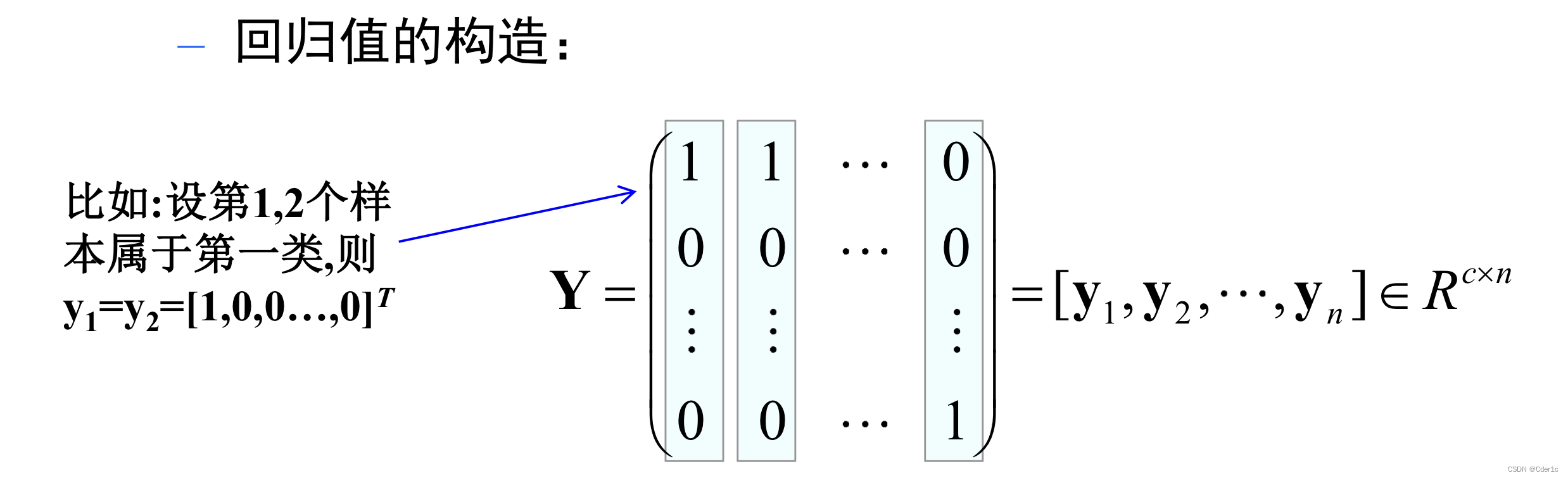
目标函数:
m
i
n
W
,
b
∑
i
=
1
n
∣
∣
W
T
x
+
b
−
y
i
∣
2
2
min_{W,b}\sum_{i=1}^{n}||W^{T}x+b-y_i|^2_2
minW,b∑i=1n∣∣WTx+b−yi∣22
∑
i
=
1
n
∣
∣
W
T
x
+
b
−
y
i
∣
2
2
=
∣
∣
W
^
T
X
^
−
Y
∣
∣
F
2
\sum_{i=1}^{n}||W^{T}x+b-y_i|^2_2=||\hat{W}^{T}\hat{X}-Y||_F^2
∑i=1n∣∣WTx+b−yi∣22=∣∣W^TX^−Y∣∣F2
得到:
W
^
=
(
X
^
X
^
T
+
λ
I
)
−
1
X
^
Y
T
∈
R
(
d
+
1
)
∗
c
\hat{W}=(\hat{X}\hat{X}^{T}+\lambda I)^{-1}\hat{X}Y^{T}\in R^{(d+1)*c}
W^=(X^X^T+λI)−1X^YT∈R(d+1)∗c
代码实现
# Define the multiple classed test function
# Input: w, a
#   w: [[class1], [class2], ...]
#   a: the parameters (sample_d+1, class_n)
# Output: f_ratio
#   f_ratio: false ratio
def multi_class_mse_test(w, a):
    w_ = copy.deepcopy(w)
    cnt = 0

    for class_i, sample in enumerate(w_):
        print(sample)
        for sample_i, test_sample in enumerate(sample):
            test_sample.append(1)
            test_sample = np.array(test_sample)
            print(np.matmul(a.T, test_sample))
            test_result = np.argmax(np.matmul(a.T, test_sample))
            if test_result != class_i:
                cnt += 1

    f_ratio = cnt / ((class_i+1)*(sample_i+1))

    print("The false rate is {} ".format(f_ratio))

    return f_ratio
代码汇总
import numpy as np
import matplotlib.pyplot as plt
import copy


# Sample w1, w2, w3, w4
w1 = [[0.1, 1.1],   [6.8, 7.1],   [-3.5, -4.1], [2.0, 2.7],   [4.1, 2.8],   [3.1, 5.0],   [-0.8, -1.3], [0.9, 1.2],   [5.0, 6.4],   [3.9, 4.0]]
w2 = [[7.1, 4.2],   [-1.4, -4.3], [4.5, 0.0],   [6.3, 1.6],   [4.2, 1.9],   [1.4, -3.2],  [2.4, -4.0],  [2.5, -6.1],  [8.4, 3.7],   [4.1, -2.2]]
w3 = [[-3.0, -2.9], [0.5, 8.7],   [2.9, 2.1],   [-0.1, 5.2],  [-4.0, 2.2],  [-1.3, 3.7],  [-3.4, 6.2],  [-4.1, 3.4],  [-5.1, 1.6],  [1.9, 5.1]]
w4 = [[-2.0, -8.4], [-8.9, 0.2],  [-4.2, -7.7], [-8.5, -3.2], [-6.7, -4.0], [-0.5, -9.2], [-5.3, -6.7], [-8.7, -6.4], [-7.1, -9.7], [-8.0, -6.3]]


# Generate the normalized augmented samples
# Input: w1, w2
#   w1: samples in class 1
#   w2: samples in class 2
# Output: w
#   w: normalized augmented samples in class 1 and a
def trans_sample(w1,w2):
    w_1 = copy.deepcopy(w1)
    w_2 = copy.deepcopy(w2)

    # Augmentation
    for sample in w_1:
        sample.append(1)
    for sample in w_2:
        sample.append(1)

    # Regulation
    w_1 = np.array(w_1)
    w_2 = -np.array(w_2)
    w   = np.concatenate([w_1, w_2])

    return w


# Define batch perception algorithm
# Input: w1, w2
#   w1: Samples in class 1
#   w2: Samples in class 2
# Output: a, n
#   a: the parameters
#   n: number of iterations
def batch_perception(w1, w2):
    # Generate the normalized augmented samples
    w = trans_sample(w1, w2)

    # Initiation
    a = np.zeros_like(w[1])
    eta = 1                             # Learning rate
    theta = np.zeros_like(w[1])+1e-6    # Termination conditions
    n = 0                               # Number of iterations

    # Implement the algorithm
    while True:
        y = np.zeros_like(w[1])
        for sample in w:
            if np.matmul(a.T, sample) <= 0:
                # the sample is misclassified
                y += sample
        eta_y = eta * y

        if all(np.abs(eta_y)<=theta):
            # if the termination conditions are satisfied, terminate the iteration
            break

        a += eta_y
        n += 1

    print ("The dicision surface a is {}\nThe number of iterations is {}.".format(a, n))
    return a, n


# Define Ho-Kashyap algorithm
# Input: w1, w2
#   w1: Samples in class 1
#   w2: Samples in class 2
# Output: a, b, n
#   a, b: the parameters
#   e: training errors
def HK_algorithm(w1, w2):
    # Generate the normalized augmented samples
    w = trans_sample(w1, w2)

    # Initiation
    a = np.zeros_like(w[1])
    b = np.zeros(w.shape[0]) + 0.5
    yita = 0.5                          # learning rate
    th_b = np.zeros(w.shape[0]) + 1e-6  # Termination condition of b
    th_n = 10000                        # Termination condition of n
    n = 0                               # Number of iterations

    # Implement the algorithm
    while n <= th_n:
        e = np.matmul(w, a) - b
        e_ = 0.5 * (e + np.abs(e))
        b += 2 * (yita) * e_
        a = np.matmul(np.matmul(np.linalg.inv(np.matmul(w.T, w)), w.T), b)
        n += 1

        if all(np.abs(e) == 0):
            # if the errors are all 0, terminate the iteration
            print ("The dicision surface a is {}.".format(a))
            print ("The dicision errors are {}.".format(e))
            return a, b, e
        if all(np.abs(e) <= th_b):
            # if the termination conditions are satisfied, terminate the iteration
            print ("The dicision surface a is {}.".format(a))
            print ("The dicision errors are {}.".format(e))
            return a, b, e

    # if the termination conditions are not satisfied when n = th_n, terminate the iteration
    print ("Iteration exceed the maxinum number! No solution found !")
    print ("The current dicision surface a is {}.".format(a))
    print ("The current dicision errors are {}.".format(e))
    return a, b, e


# Define multiple class MSE algorithm
# Input: w
#   w: [[class1], [class2], ...]
# Output: a
#   a: the parameters (sample_d+1, class_n)
def multi_class_mse(w_i):
    w_ = copy.deepcopy(w_i)
    class_n = len(w_)
    sample_n = len(w_[0])

    # Initiation
    w = []
    y = np.zeros((class_n, class_n*sample_n))
    for class_idx, class_sample in enumerate(w_):
        for sample in class_sample:
            sample.append(1)
            w.append(sample)
        y[class_idx, class_idx*sample_n:(class_idx+1)*sample_n] = 1
    print(y)
    w = np.array(w).T

    # w: (class_n*sample_n, 3)
    # y: (class_n, class_n*sample_n)
    a = np.matmul(np.matmul(np.linalg.inv(np.matmul(w, w.T)+0.01), w), y.T)

    print ("The dicision surface a is {}.".format(a))
    return a


# Define the multiple classed test function
# Input: w, a
#   w: [[class1], [class2], ...]
#   a: the parameters (sample_d+1, class_n)
# Output: f_ratio
#   f_ratio: false ratio
def multi_class_mse_test(w, a):
    w_ = copy.deepcopy(w)
    cnt = 0

    for class_i, sample in enumerate(w_):
        print(sample)
        for sample_i, test_sample in enumerate(sample):
            test_sample.append(1)
            test_sample = np.array(test_sample)
            print(np.matmul(a.T, test_sample))
            test_result = np.argmax(np.matmul(a.T, test_sample))
            if test_result != class_i:
                cnt += 1

    f_ratio = cnt / ((class_i+1)*(sample_i+1))

    print("The false rate is {} ".format(f_ratio))

    return f_ratio


# Show the classification results
# Input: w1, w2
#   w1: Samples in class 1
#   w2: Samples in class 2
#   a: the parameters
def show_result(w1, w2, a):
    # Samples in class 1
    w_1 = np.array(w1)
    x1 = w_1[:, 0]
    y1 = w_1[:, 1]
    plt.scatter(x1, y1, marker = '.',color = 'red')

    # Samples in class 2
    w_2 = np.array(w2)
    x2 = w_2[:, 0]
    y2 = w_2[:, 1]
    plt.scatter(x2, y2, marker = '.',color = 'blue')

    # Decision surface
    x = np.arange(-10, 10, 0.1)
    y = -a[0]/a[1]*x - a[2]/a[1]
    plt.plot(x, y)

    plt.xlabel('x_1')
    plt.ylabel('x_2')
    plt.title('Classfication Result')
    plt.show()


# Show the multiple classification results
# Input: w, a
#   w: [[class1], [class2], ...]
#   a: the parameters
def multi_class_show_result(w, a):
    class_n = len(w)

    for class_idx, class_sample in enumerate(w):
        # Samples in class_idx
        w_i = np.array(class_sample)
        x = w_i[:, 0]
        y = w_i[:, 1]
        plt.scatter(x, y)

        # Decision surface
        x = np.arange(-10, 10, 0.1)
        y = -a[0][class_idx]/a[1][class_idx]*x - a[2][class_idx]/a[1][class_idx]
        plt.plot(x, y)

    plt.xlabel('x_1')
    plt.ylabel('x_2')
    plt.title('Classfication Result')
    plt.show()


if __name__ == "__main__":
    print("The result of the batch perception algorithm is shown below")
    print("w1 and w2")
    a, n = batch_perception(w1, w2)
    show_result(w1, w2, a)
    print("w3 and w2")
    a, n = batch_perception(w3, w2)
    show_result(w3, w2, a)

    print("-------------------------------------")
    print("The result of the Ho-Kashyap algorithm is shown below")
    print("w1 and w3")
    a, b, e = HK_algorithm(w1, w3)
    show_result(w1, w3, a)
    print("w2 and w4")
    a, b, e = HK_algorithm(w2, w4)
    show_result(w2, w4, a)

    print("-------------------------------------")
    print("The result of the multiple calss MSE is shown below")
    a = multi_class_mse([w1[:8], w2[:8], w3[:8], w4[:8]])
    multi_class_show_result([w1[:8], w2[:8], w3[:8], w4[:8]], a)
    multi_class_mse_test([w1[8:], w2[8:], w3[8:], w4[8:]], a)


 被折叠的 条评论
为什么被折叠?
被折叠的 条评论
为什么被折叠?
 到【灌水乐园】发言


