


 该项目结合历史使用模式与天气数据,预测华盛顿特区自行车租赁需求。先收集Kaggle数据,对其进行预处理和分析,发现天气、时间等因素对租借数有影响。提取9个特征,采用多种模型建模预测,默认随机森林和简单参数神经网络R方得分较高,调参后预测结果有所提升。
一、提出问题
在本项目中,参与者被要求将历史使用模式与天气数据相结合,以便预测华盛顿特区的自行车租赁计划中的自行车租赁需求。
二、理解数据
2.1 收集数据
一般而言,数据由甲方提供。若甲方不提供数据,则需要根据相关问题从网络爬取,或者以问卷调查形式收集。本次共享单车数据分析项目数据源于Kaggle。获取数据后需要对数据整体进行分析,从而提炼问题,为后续建模奠定基础。
首先查看Kaggle所提供的数据描述:
(1) 日期时间:年/月/日/时间,例:2011/1/1 0:00
(2) 季节:1=春,2=夏,3=秋天,4=冬天
(3) 假日:是否是节假日(0=否,1=是)
(4) 工作日:是否是工作日(0=否,1=是)
(5) 天气:1=晴天、多云等(良好),2=阴天薄雾等(普通),3=小雪、小雨等(稍差),4=大雨、冰雹等(极差)
(6) 实际温度(℃)
(7) 感觉温度(℃)
(8) 湿度
(9) 风速
(10)未注册用户租借数量
(11)注册用户租借数量
(12)总租借数量
根据官方数据描述,特征为前9项,分别为日期时间(1)、季节(2)、工作日/节假日(3-4)、天气(5-9)四类;标签为后3项:注册/未注册用户租借数量以及租借总数。因为官方规定的提交文件中要求预测的只有租借总数,因此本项目中只关注租借总数的预测。
2.2导入并理解数据
首先导入并查看训练数据和测试数据:
-
import pandas
as pd
-
#导入并查看训练数据和测试数据
-
train_data = pd.read_csv(
‘data/train.csv’)
-
test_data = pd.read_csv(
‘data/test.csv’)
-
print(train_data.shape)
-
print(train_data.info())
-
print(test_data.shape)
-
print(test_data.info())
训练数据共12列,10886行,测试数据共9列,6493行,且所有数据完整,没有缺失。相比于训练数据,测试数据缺少注册/未注册用户租借数量以及租借总数3个标签,需要我们通过建模进行预测。
三、数据处理与分析
3.1 数据预处理
在数据处理过程中,最好将训练数据与测试数据合并在一起处理,方便特征的转换。通过查看数据,训练和测试数据均无缺失、不一致和非法等问题。值得注意的是,日期时间特征由年、月、日和具体小时组成,还可以根据日期计算其星期,因此可以将日期时间拆分成年、月、日、时和星期5个特征。
-
#第二步:数据预处理
-
#合并两种数据,使之共同进行数据规范化
-
data = train_data.append(test_data)
-
#拆分年、月、日、时
-
data[
‘year’] = data.datetime.apply(
lambda x: x.split()[
0].split(
’-’)[
0])
-
data[
‘year’] = data[
‘year’].apply(
lambda x: int(x))
-
data[
‘month’] = data.datetime.apply(
lambda x: x.split()[
0].split(
’-’)[
1])
-
data[
‘month’] = data[
‘month’].apply(
lambda x: int(x))
-
data[
‘day’] = data.datetime.apply(
lambda x: x.split()[
0].split(
’-’)[
2])
-
data[
‘day’] = data[
‘day’].apply(
lambda x: int(x))
-
data[
‘hour’] = data.datetime.apply(
lambda x: x.split()[
1].split(
’:’)[
0])
-
data[
‘hour’] = data[
‘hour’].apply(
lambda x: int(x))
-
data[
‘date’] = data.datetime.apply(
lambda x: x.split()[
0])
-
data[
‘weekday’] = pd.to_datetime(data[
‘date’]).dt.weekday_name
-
data[
‘weekday’] = data[
‘weekday’].map({
‘Monday’:
1,
‘Tuesday’:
2,
‘Wednesday’:
3,
-
‘Thursday’:
4,
‘Friday’:
5,
‘Saturday’:
6,
‘Sunday’:
7})
-
data = data.drop(
‘datetime’,axis=
1)
-
#重新安排整体数据的特征
-
cols = [
‘year’,
‘month’,
‘day’,
‘weekday’,
‘hour’,
‘season’,
‘holiday’,
‘workingday’,
‘weather’,
‘temp’,
‘atemp’,
-
‘humidity’,
‘windspeed’,
‘casual’,
‘registered’,
‘count’]
-
data = data.ix[:,cols]
-
#分离训练数据与测试数据
-
train = data.iloc[:
10886]
-
test = data.iloc[
10886:]
3.2 数据分析
规范数据后,快速查看各影响因素对租借数的影响:
-
#第三步:特征工程
-
#1、计算相关系数,并快速查看
-
correlation = train.corr()
-
influence_order = correlation[
‘count’].sort_values(ascending=
False)
-
influence_order_abs = abs(correlation[
‘count’]).sort_values(ascending=
False)
-
print(influence_order)
-
print(influence_order_abs)

从相关系数可以看出,天气(包括温度、湿度)对租借数存在明显影响,其中temp和atemp的意义及其与count的相关系数十分接近,因此可以只取atemp作为温度特征。此外,year、month、season等时间因素对count也存在明显影响,而holiday和weekday与count的相关系数极小。
为了更加直观地展现所有特征之间的影响,作相关系数热力图:
-
#2、作相关性分析的热力图
-
import matplotlib.pyplot
as plt
-
import seaborn
as sn
-
f,ax = plt.subplots(figsize=(
16,
16))
-
cmap = sn.cubehelix_palette(light=
1,as_cmap=
True)
-
sn.heatmap(correlation,annot=
True,center=
1,cmap=cmap,linewidths=
1,ax=ax)
-
sn.heatmap(correlation,vmax=
1,square=
True,annot=
True,linewidths=
1)
-
plt.show()

接下来,深入分析各特征对租借数的影响规律,对每个特征进行可视化:
-
#3、每个特征对租借量的影响
-
#(1) 时间维度——年份
-
sn.boxplot(train[
‘year’],train[
‘count’])
-
plt.title(
“The influence of year”)
-
plt.show()
-
#(2) 时间维度——月份
-
sn.pointplot(train[
‘month’],train[
‘count’])
-
plt.title(
“The influence of month”)
-
plt.show()
-
#(3) 时间维度——季节
-
sn.boxplot(train[
‘season’],train[
‘count’])
-
plt.title(
“The influence of season”)
-
plt.show()
-
#(4) 时间维度——时间(小时)
-
sn.barplot(train[
‘hour’],train[
‘count’])
-
plt.title(
“The influence of hour”)
-
plt.show()
(1)年份对租借数的影响
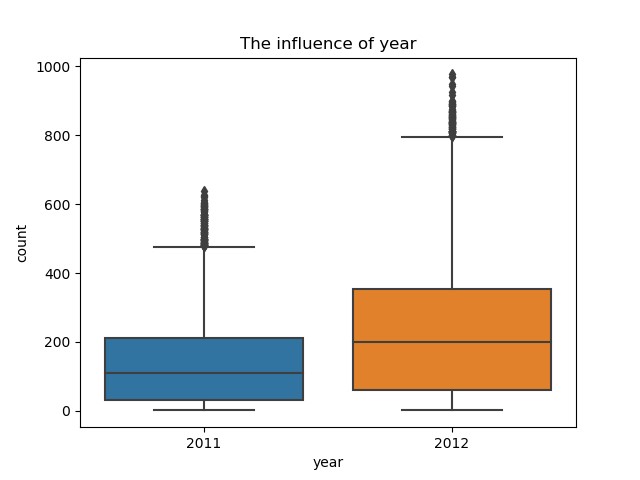
2012年的租借数明显比2011年高,说明随着时间的推移,共享单车逐渐被更多的人熟悉和认可,使用者越来越多。
(2)月份对租借数的影响

月份对租借数影响显著,从1月份开始每月的租借数快速增加,到6月份达到顶峰,随后至10月缓慢降低,10月后急剧减少。这明显与季节有关。
(3)季节对租借数的影响

通过各季度箱型图可以看出季节对租借数的影响符合预期:春季天气仍然寒冷,骑车人少;随着天气转暖,骑车人逐渐增多,并在秋季(天气最适宜时)达到顶峰;随后进入冬季,天气变冷,骑车人减少。
因为月份和季节对租借数的影响重合,且月份更加详细,因此在随后的建模过程中选取月份特征,删除季节特征。
(4)时间(小时)对租借数的影响
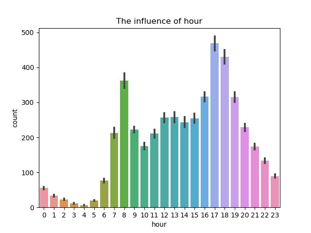
从时间的分布上来看,每天有两个高峰期,分别是早上8点左右和下午17点左右,正好是工作日的上下班高峰期。而介于两者之间的白天时间变化规律不明显,可能与节假日有关,因此以此为基础需要考虑节假日和星期的影响。
-
#星期、节假日和工作日的影响
-
fig, axes = plt.subplots(
2,
1,figsize=(
16,
10))
-
ax1 = plt.subplot(
2,
1,
1)
-
sn.pointplot(train[
‘hour’],train[
‘count’],hue=train[
‘weekday’],ax=ax1)
-
ax1.set_title(
“The influence of hour (weekday)”)
-
ax2 = plt.subplot(
2,
2,
3)
-
sn.pointplot(train[
‘hour’],train[
‘count’],hue=train[
‘workingday’],ax=ax2)
-
ax2.set_title(
“The influence of hour (workingday)”)
-
ax3 = plt.subplot(
2,
2,
4)
-
sn.pointplot(train[
‘hour’],train[
‘count’],hue=train[
‘holiday’],ax=ax3)
-
ax3.set_title(
“The influence of hour (holiday)”)
-
plt.show()
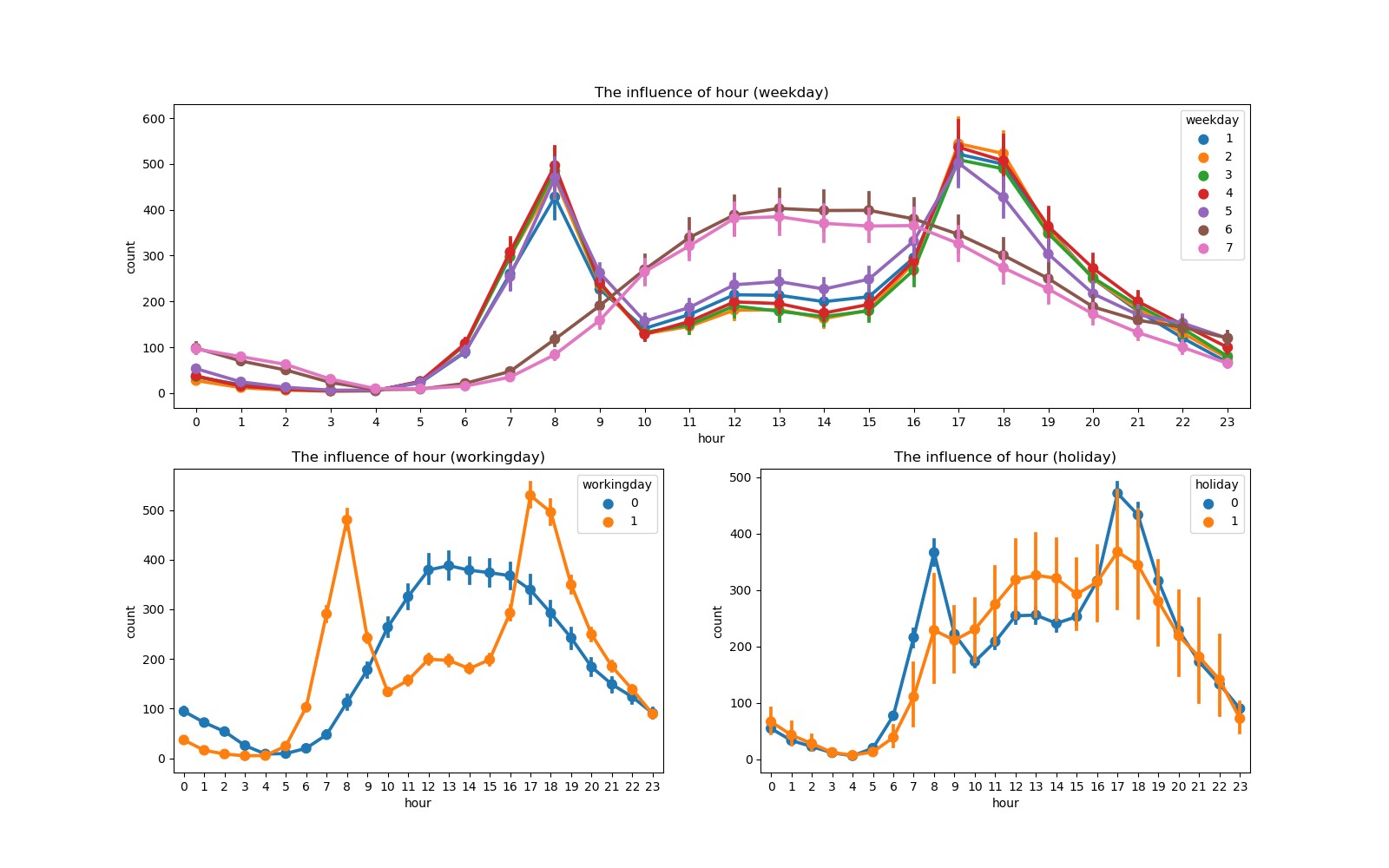
可以看出,工作日早晚上班高峰期租借量高,其余时间租借量低;节假日中午及午后租借量较高,符合节假日人们出行用车的规律。
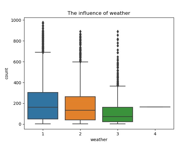
(5)天气对租借数的影响
-
#(5) 天气的影响
-
sn.boxplot(train[
‘weather’],train[
‘count’])
-
plt.title(
“The influence of weather”)
-
plt.show()
(6)具体天气因素(温度、湿度和风速)的影响
-
#(6) 温度、湿度、风速的影响
-
cols = [
‘temp’,
‘atemp’,
‘humidity’,
‘windspeed’,
‘count’]
-
sn.pairplot(train[cols])
-
plt.show()
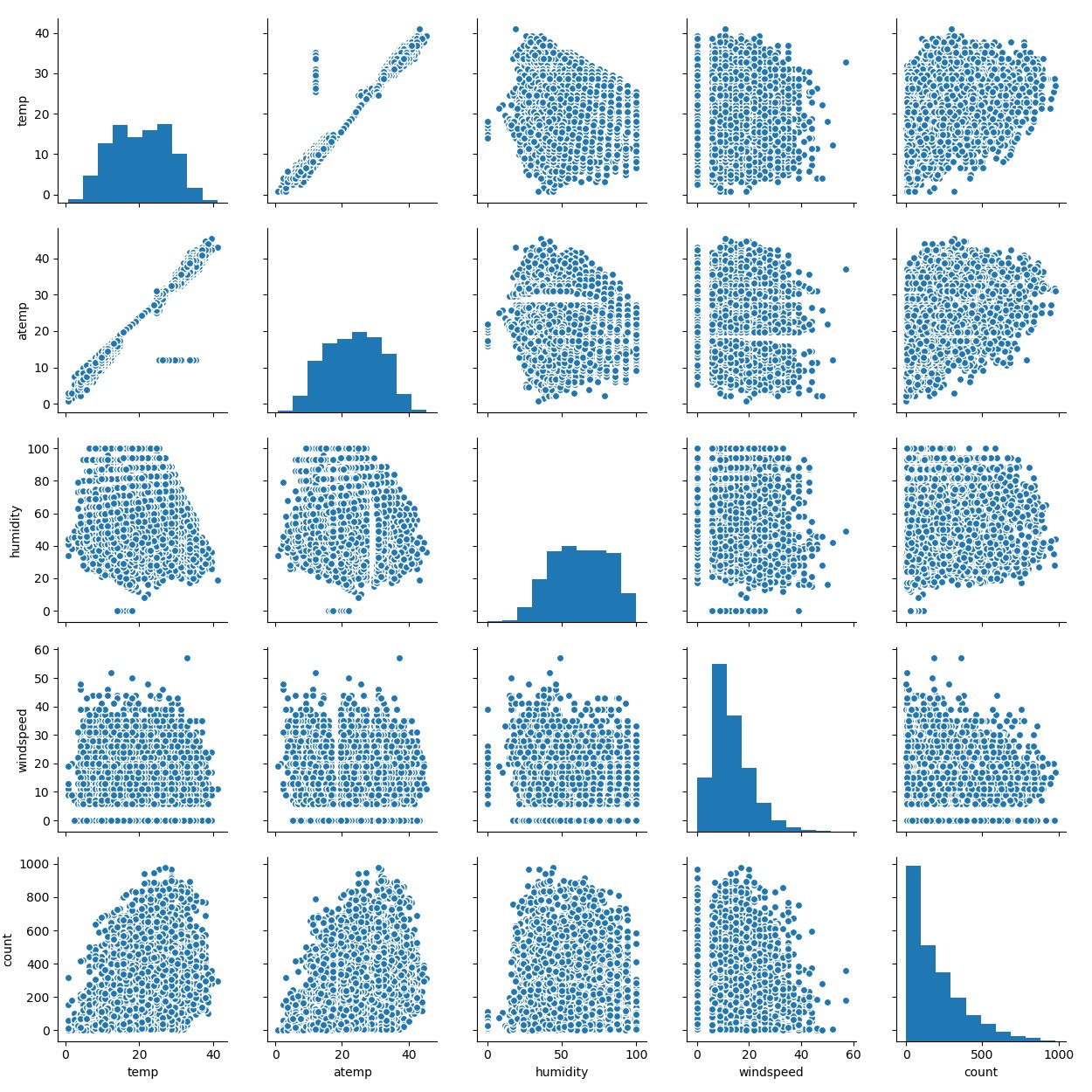
作出多个连续变量之间的相关图,可以比较任意两个连续变量之间的关系。图中可以明显看出temp和atemp大致成线性关系,但也存在一组数据显著偏离线性相关趋势,可能与湿度和风速有关。因此,可以认为temp、humidity和windspeed三者共同决定了atemp,因此在后续建模过程中可以删除atemp特征。
进一步研究温度、湿度和风速对租借数的影响:
-
fig, axes = plt.subplots(
1,
3,figsize=(
24,
8))
-
ax1 = plt.subplot(
1,
3,
1)
-
ax2 = plt.subplot(
1,
3,
2)
-
ax3 = plt.subplot(
1,
3,
3)
-
sn.regplot(train[
‘temp’],train[
‘count’],ax=ax1)
-
sn.regplot(train[
‘humidity’],train[
‘count’],ax=ax2)
-
sn.regplot(train[
‘windspeed’],train[
‘count’],ax=ax3)
-
ax1.set_title(
“The influence of temperature”)
-
ax2.set_title(
“The influence of humidity”)
-
ax3.set_title(
“The influence of windspeed”)
-
plt.show()

虽然三种天气因素对租借数的影响比较分散,但可以明显看出温度和风速与租借数成正相关,湿度与租借数成负相关。
3.3 特征工程
综上所述,本项目提取特征year、month、hour、workingday、holiday、weather、temp、humidity和windspeed共9个特征预测租借总数。其中year、month、hour、workingday、holiday和weather为离散量,且由于workingday和holiday已经是二元属性,因此其余四个需要进行独热编码(one-hot)方式进行转换。
-
#特征工程
-
#所选取的特征:year、month、hour、workingday、holiday、weather、temp、humidity和windspeed
-
#(1) 删除不要的变量
-
data = data.drop([
‘day’,
‘weekday’,
‘season’,
‘atemp’,
‘casual’,
‘registered’],axis=
1)
-
#(2) 离散型变量(year、month、hour、weather)转换
-
column_trans = [
‘year’,
‘month’,
‘hour’,
‘weather’]
-
data = pd.get_dummies(data, columns=column_trans)
四、构建模型
接下来,需要对数据进行建模预测,分别采用三种典型集成学习模型(普通随机森林、极端随机森林模型和梯度提升树模型)、XGBoost模型和人工神经网络模型。此处均采用模型的默认参数或简单参数,如人工神经网络选用三层神经网络,每层包含神经元数量相同,且均为特征个数。
-
#机器学习
-
#1、特征向量化
-
col_trans = [
‘holiday’,
‘workingday’,
‘temp’,
‘humidity’,
‘windspeed’,
-
‘year_2011’,
‘year_2012’,
‘month_1’,
‘month_2’,
‘month_3’,
‘month_4’,
-
‘month_5’,
‘month_6’,
‘month_7’,
‘month_8’,
‘month_9’,
‘month_10’,
-
‘month_11’,
‘month_12’,
‘hour_0’,
‘hour_1’,
‘hour_2’,
‘hour_3’,
-
‘hour_4’,
‘hour_5’,
‘hour_6’,
‘hour_7’,
‘hour_8’,
‘hour_9’,
‘hour_10’,
-
‘hour_11’,
‘hour_12’,
‘hour_13’,
‘hour_14’,
‘hour_15’,
‘hour_16’,
-
‘hour_17’,
‘hour_18’,
‘hour_19’,
‘hour_20’,
‘hour_21’,
‘hour_22’,
-
‘hour_23’,
‘weather_1’,
‘weather_2’,
‘weather_3’,
‘weather_4’]
-
X_train = data[col_trans].iloc[:
10886]
-
X_test = data[col_trans].iloc[
10886:]
-
Y_train = data[
‘count’].iloc[:
10886]
-
from sklearn.feature_extraction
import DictVectorizer
-
vec = DictVectorizer(sparse=
False)
-
X_train = vec.fit_transform(X_train.to_dict(orient=
‘record’))
-
X_test = vec.fit_transform(X_test.to_dict(orient=
‘record’))
-
-
#分割训练数据
-
from sklearn.model_selection
import train_test_split
-
x_train, x_test, y_train, y_test = train_test_split(X_train, Y_train, test_size=
0.25, random_state=
40)
-
-
#2、建模预测,分别采用常规集成学习方法、XGBoost和神经网络三大类模型
-
from sklearn.ensemble
import RandomForestRegressor
-
from sklearn.ensemble
import ExtraTreesRegressor
-
from sklearn.ensemble
import GradientBoostingRegressor
-
from xgboost
import XGBRegressor
-
from sklearn.neural_network
import MLPRegressor
-
from sklearn.metrics
import r2_score
-
-
#(1)集成学习方法——普通随机森林
-
rfr = RandomForestRegressor()
-
rfr.fit(x_train,y_train)
-
#print(rfr.fit(x_train,y_train))
-
rfr_y_predict = rfr.predict(x_test)
-
print(
“集成学习方法——普通随机森林回归模型的R方得分为:”,r2_score(y_test,rfr_y_predict))
-
-
#(2)集成学习方法——极端随机森林
-
etr = ExtraTreesRegressor()
-
etr.fit(x_train,y_train)
-
#print(etr.fit(x_train,y_train))
-
etr_y_predict = etr.predict(x_test)
-
print(
“集成学习方法——极端随机森林回归模型的R方得分为:”,r2_score(y_test,etr_y_predict))
-
-
#(3)集成学习方法——梯度提升树
-
gbr = GradientBoostingRegressor()
-
gbr.fit(x_train,y_train)
-
#print(gbr.fit(x_train,y_train))
-
gbr_y_predict = gbr.predict(x_test)
-
print(
“集成学习方法——梯度提升树回归模型的R方得分为:”,r2_score(y_test,gbr_y_predict))
-
-
#(4) XGBoost回归模型
-
xgbr = XGBRegressor()
-
xgbr.fit(x_train,y_train)
-
#print(xgbr.fit(x_train,y_train))
-
xgbr_y_predict = xgbr.predict(x_test)
-
print(
“XGBoost回归模型的R方得分为:”,r2_score(y_test,xgbr_y_predict))
-
-
#(5) 神经网络回归模型
-
mlp = MLPRegressor(hidden_layer_sizes=(
47,
47,
47),max_iter=
500)
-
mlp.fit(x_train,y_train)
-
mlp_y_predict = mlp.predict(x_test)
-
print(
“神经网络回归模型的R方得分为:”,r2_score(y_test,mlp_y_predict))
最终模型预测能力如下:

可以看出,默认配置的随机森林模型和简单参数的人工神经网络R方得分较高。分别采用极端随机森林模型和人工神经网络预测测试数据,上传至Kaggle评分,两者结果相似,其中极端随机森林模型的效果略好,结果如下:

本项目的得分为均方根对数误差(RMSLE),值越小越好。该比赛官方记录最好得分为0.33756。因此,该模型还有待提高,主要是对模型进行调参。每种机器学习模型均有若干参数,需理解每个参数的意义和作用,采用适当方法进行调参,以期获得最佳参数,提高预测准确率。
下面以极端随机森林模型为例,进行调参。需要了解模型参数及调参步骤,该部分内容已在另一篇原创文章中详细阐述:https://blog.csdn.net/Caesar1993_Wang/article/details/80337103
最终通过调参,获得最佳参数(random_state=27,n_estimators=41,max_depth=38,max_features=14),预测结果也有所提高:

本项目基本流程已经结束,但还有许多可以改进的地方:分别预测注册和未注册的租借数;对连续性特征量进行归一化;使用神经网络对预测模型的参数进行大规模调参。


 303
303

 被折叠的 条评论
为什么被折叠?
被折叠的 条评论
为什么被折叠?
 到【灌水乐园】发言


