常见的地图绘制方法，这个包全包了~~

在上一篇介绍完Bokeh精美可视化作品之后，有小伙伴咨询我能不能稍系统的介绍下如何在地图上添加如柱形图等其他元素的付方法？ 这就让我想到一个优秀的地图绘制可视化包-R-cartography，虽然之前也有简单介绍过，本期就具体分享下该包绘制的地图可视化作品(我们大部分绘图所使用的数据都是基于该包自带)。主要内容涉及以下两个部分：

• cartography 特征

• cartography 图层介绍

• cartography 实例绘制

• 更多详细的数据可视化教程，可订阅我们的店铺课程：

• 

cartography 特征

1. Symbology

地图图层绘制函数，也是cartography最重要的绘图函数之一。每个功能着重于一个单一的制图表达(例如，比例符号或合计表示)，并将其显示在地理参考图上。该解决方案允许将每个表示视为一个图层，并将多个表示覆盖在同一地图上。每个函数都有两个主要参数：

• x：空间对象（最好是sf对象。

• var：要映射的变量的名称。

如果变量包含在SpatialDataFrame中，则通过spdf参数处理sp对象；如果变量位于需要连接到SpatialDataFrame的单独data.frame中，则通过spdf，spdfid，df，dfid处理sp对象。

2. Transformations

一组功能专用于空间对象的创建或转换（例如边界提取，网格或链接创建）。提供这些功能是为了简化一些通常需要地理处理的高级地图的创建。

3. Map Layout

除了制图功能外，还有一些其他功能专用于布局设计（例如，可自定义的比例尺，向北箭头，标题，来源或作者信息…）。

4. Color Palettes

包装内随附16种原始调色板。可以定制和组合这些调色板。

5. Legends

图例默认沿制图图层显示，但Legend*（）函数可提供更多参数。

6. Classification

getBreaks（）可以访问用于数据装箱的大多数分类方法(本期推文主要介绍地图绘制相关内容，这部分不做介绍)。

cartography 图层功能介绍

cartography包提供了提供了许多优秀且功能强大的绘制函数用于绘制各类地图可视化作品，下面就一一介绍：

• Choropleth Layer

library(sf)
library(cartography)
mtq <- st_read(system.file("gpkg/mtq.gpkg", package="cartography"))
mtq$POPDENS <- 1e6 * mtq$POP / st_area(x = mtq)
# Default
choroLayer(x = mtq, var = "POPDENS")

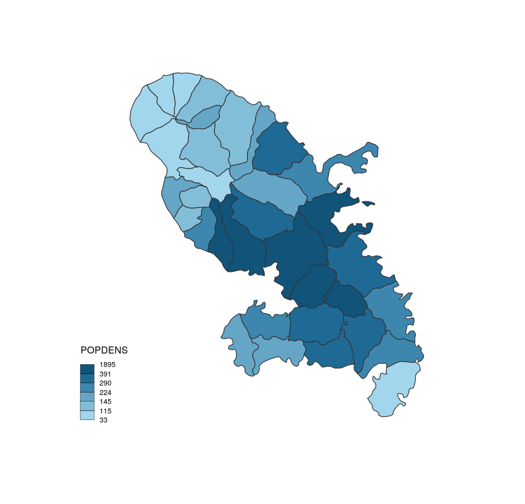
choroLayer default

# With parameters 
choroLayer(x = mtq, var = "POPDENS",
           method = "quantile", nclass = 5,
           col = carto.pal(pal1 = "sand.pal", n1 = 5),
           border = "grey40",
           legend.pos = "topright", legend.values.rnd = 0,
           legend.title.txt = "Population Density\n(people per km2)")

# Layout
layoutLayer(title = "Population Distribution in Martinique, 2015")

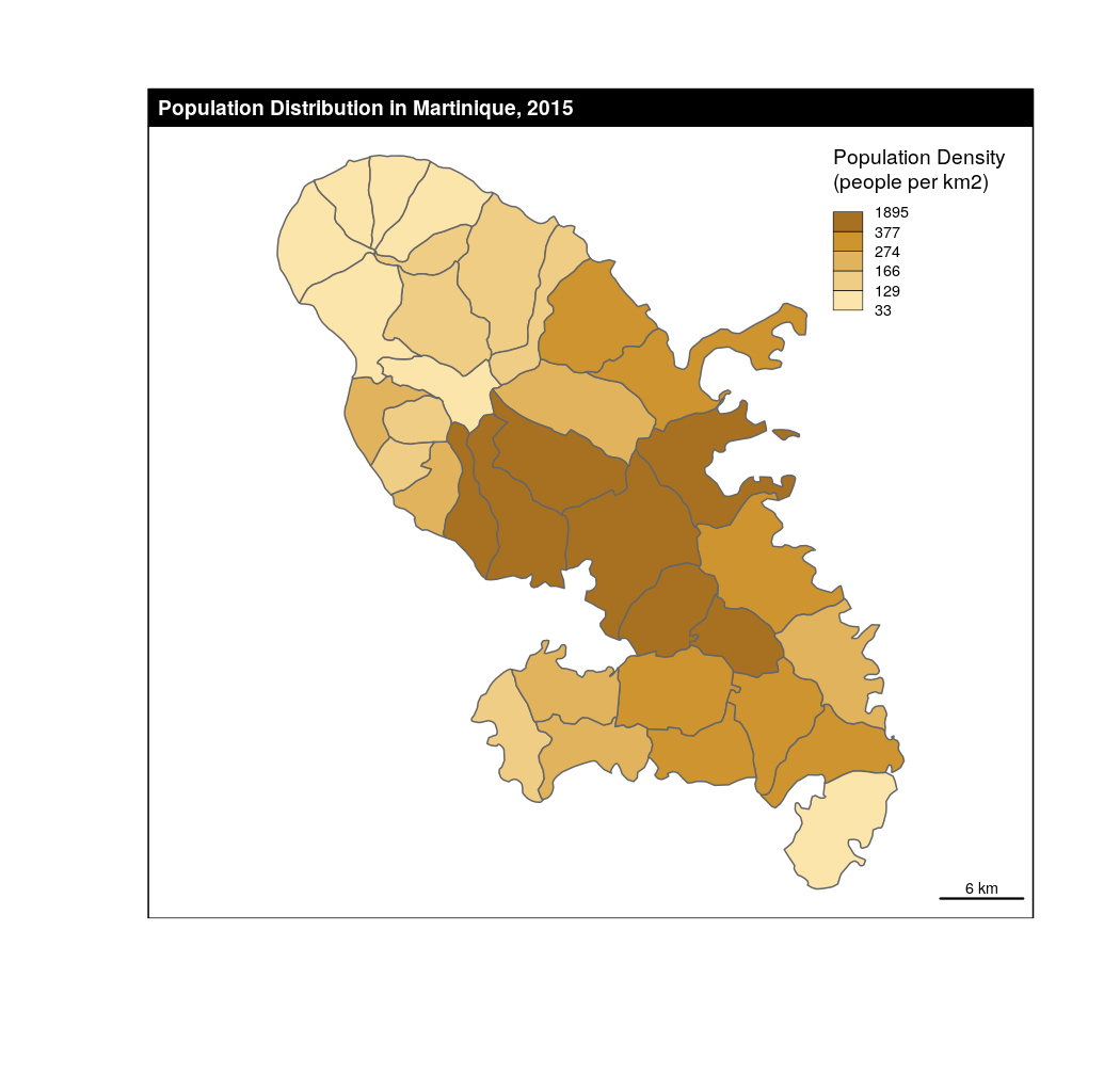
choroLayer With parameters

• Discontinuities Layer

library(sf)
mtq <- st_read(system.file("gpkg/mtq.gpkg", package="cartography"))
# Get borders
mtq.borders <- getBorders(x = mtq)
# Median Income 
choroLayer(x = mtq, var = "MED", border = "grey", lwd = 0.5,
           method = 'equal', nclass = 6, legend.pos = "topleft",
           legend.title.txt = "Median Income\n(in euros)" )
# Discontinuities
discLayer(x = mtq.borders, df = mtq,
          var = "MED", col="red4", nclass=3,
          method="equal", threshold = 0.4, sizemin = 0.5,
          sizemax = 10, type = "abs",legend.values.rnd = 0,
          legend.title.txt = "Discontinuities\n(absolute difference)",
          legend.pos = "bottomleft", add=TRUE)

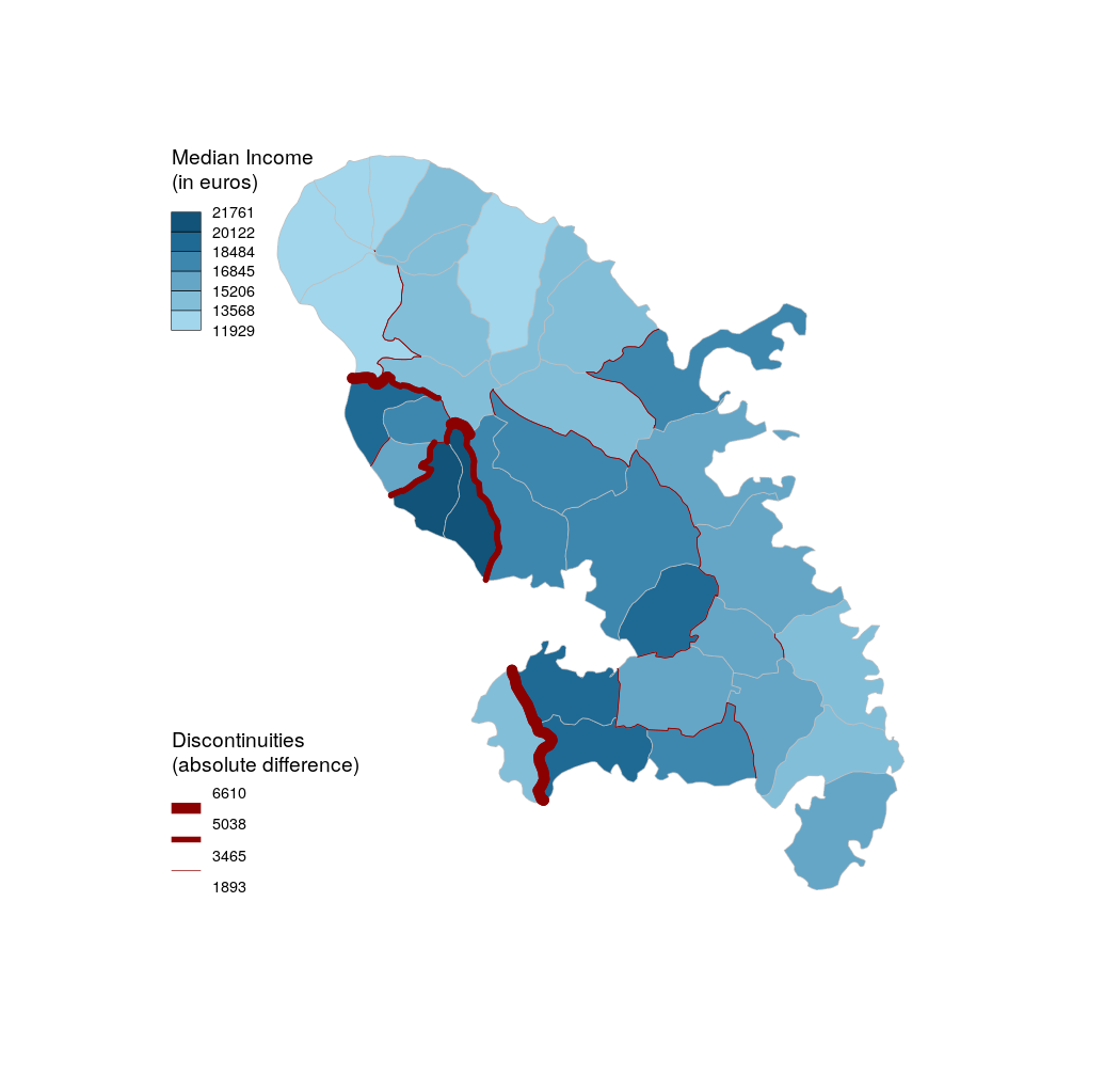
Discontinuities

• Plot a Ghost Layer

library(sf)
mtq <- st_read(system.file("gpkg/mtq.gpkg", package="cartography"))
target <- mtq[30,]
ghostLayer(target, bg = "lightblue")
plot(st_geometry(mtq), add = TRUE, col = "gold2")
plot(st_geometry(target), add = TRUE, col = "red")
# overly complicated label placement trick:
labelLayer(x = suppressWarnings(st_intersection(mtq, st_buffer(target, 2000))),
           txt = "LIBGEO", halo = TRUE, cex = .9, r = .14, font = 2,
           bg = "grey20", col= "white")

Ghost Layer

• Graduated Links Layer 该类型地图较为常用，大家可以多注意下~~

library(sf)
mtq <- st_read(system.file("gpkg/mtq.gpkg", package="cartography"))
mob <- read.csv(system.file("csv/mob.csv", package="cartography"))
# Create a link layer - work mobilities to Fort-de-France (97209)
mob.sf <- getLinkLayer(x = mtq, df = mob[mob$j==97209,], dfid = c("i", "j"))
# Plot the links - Work mobility
plot(st_geometry(mtq), col = "grey60",border = "grey20")
gradLinkLayer(x = mob.sf, df = mob,
              legend.pos = "topright",
              var = "fij",
              breaks = c(109,500,1000,2000,4679),
              lwd = c(1,2,4,10),
              col = "#92000090", add = TRUE)

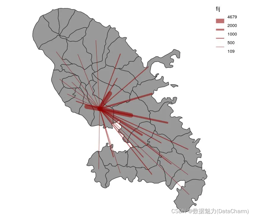
Links Layer

• Graduated and Colored Links Layer 可以看作上个图层的优化

library(sf)
mtq <- st_read(system.file("gpkg/mtq.gpkg", package="cartography"))
mob <- read.csv(system.file("csv/mob.csv", package="cartography"))
# Create a link layer - work mobilities to Fort-de-France (97209) and 
# Le Lamentin (97213)
mob.sf <- getLinkLayer(x = mtq, df = mob[mob$j %in% c(97209, 97213),],
                       dfid = c("i", "j"))
# Plot the links - Work mobility
plot(st_geometry(mtq), col = "grey60",border = "grey20")
gradLinkTypoLayer(x = mob.sf, df = mob,
                  var = "fij",
                  breaks = c(109,500,1000,2000,4679),
                  lwd = c(1,2,4,10),
                  var2='j', add = TRUE)

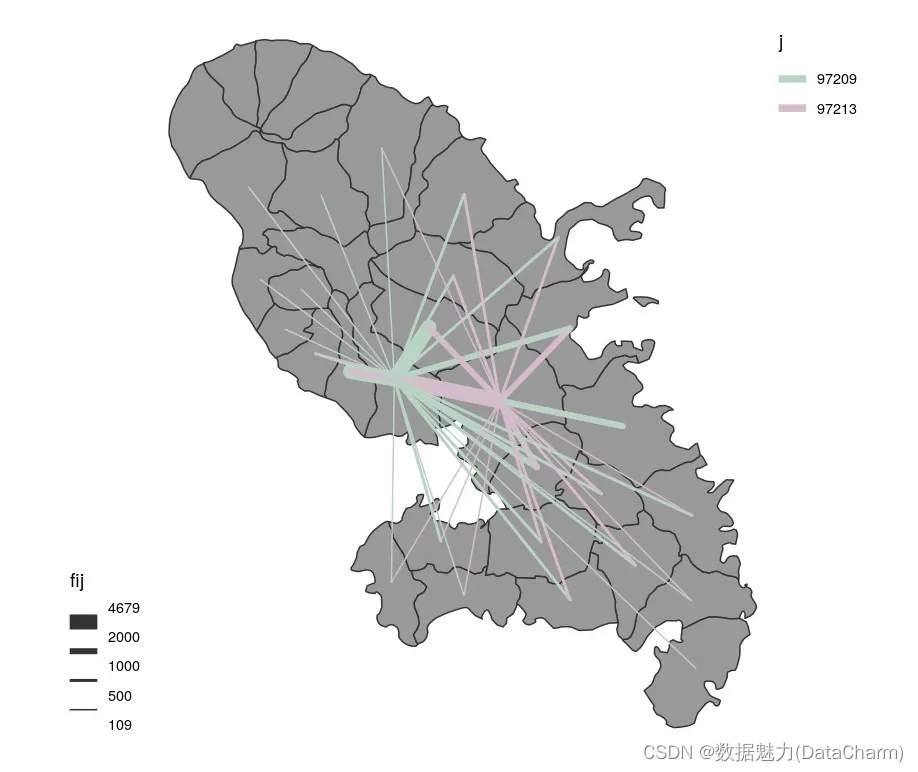
Colored Links Layer

• Hatched Layer 该图层绘制函数有多种类型，这里只介绍一种。

library(sf)
mtq <- st_read(system.file("gpkg/mtq.gpkg", package = "cartography"))
plot(st_geometry(mtq), border = NA, col="grey80")
hatchedLayer(mtq, "text", txt = "Y", add=TRUE)
title("text")

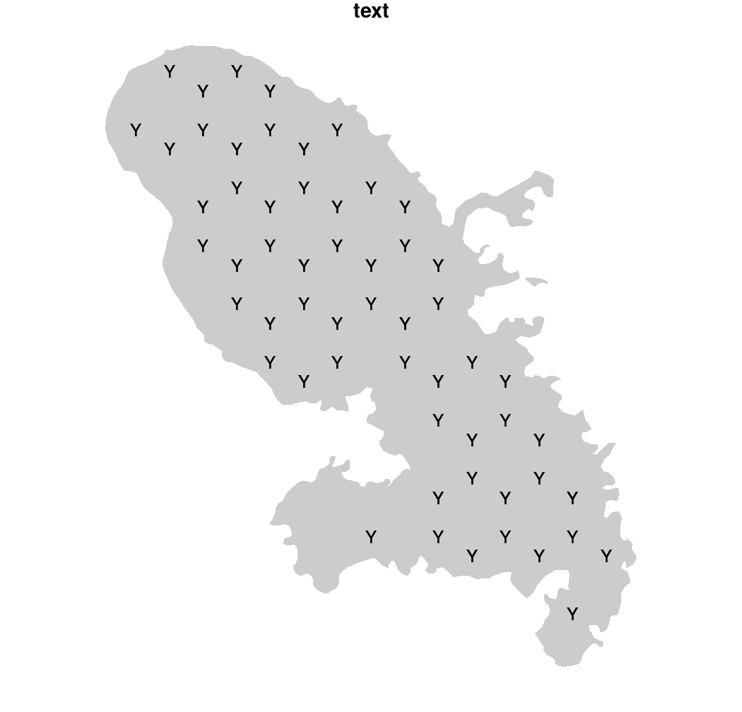
Hatched Layer text

• Label Layer

library(sf)
opar <- par(mar = c(0,0,0,0))
mtq <- st_read(system.file("gpkg/mtq.gpkg", package="cartography"))
plot(st_geometry(mtq), col = "darkseagreen3", border = "darkseagreen4",
     bg = "#A6CAE0")
labelLayer(x = mtq, txt = "LIBGEO", col= "black", cex = 0.7, font = 4,
           halo = TRUE, bg = "white", r = 0.1,
           overlap = FALSE, show.lines = FALSE)

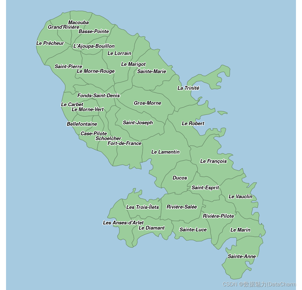
Label Layer

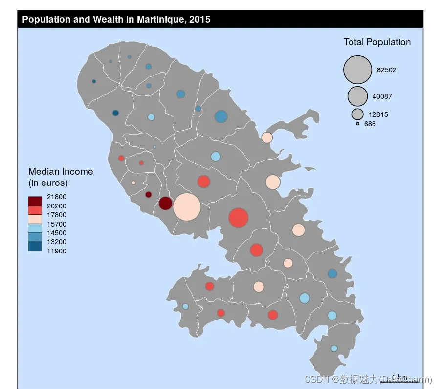
• Proportional and Choropleth Symbols Layer

library(sf)
mtq <- st_read(system.file("gpkg/mtq.gpkg", package="cartography"))
plot(st_geometry(mtq), col = "grey60",border = "white",
     lwd=0.4, bg = "lightsteelblue1")
propSymbolsChoroLayer(x = mtq, var = "POP", var2 = "MED",
                      col = carto.pal(pal1 = "blue.pal", n1 = 3,
                                      pal2 = "red.pal", n2 = 3),
                      inches = 0.2, method = "q6",
                      border = "grey50", lwd = 1,
                      legend.var.pos = "topright",
                      legend.var2.pos = "left",
                      legend.var2.values.rnd = -2,
                      legend.var2.title.txt = "Median Income\n(in euros)",
                      legend.var.title.txt = "Total Population",
                      legend.var.style = "e")
# First layout
layoutLayer(title="Population and Wealth in Martinique, 2015")

• Proportional Symbols Typo Layer

library(sf)
mtq <- st_read(system.file("gpkg/mtq.gpkg", package="cartography"))
plot(st_geometry(mtq), col = "lightblue4",border = "lightblue3",
     bg = "lightblue1")
# Population plot on proportional symbols
propSymbolsTypoLayer(x = mtq, var = "POP", var2 = "STATUS",
                     symbols = "circle",
                     col = c("aquamarine4", "yellow3","wheat"),
                     legend.var2.values.order = c("Prefecture",
                                                  "Sub-prefecture",
                                                  "Simple municipality"),
                     legend.var.pos = "right", border = "grey",
                     legend.var.title.txt = "Total\nPopulation")
layoutLayer(title = "Population Distribution in Martinique, 2015")

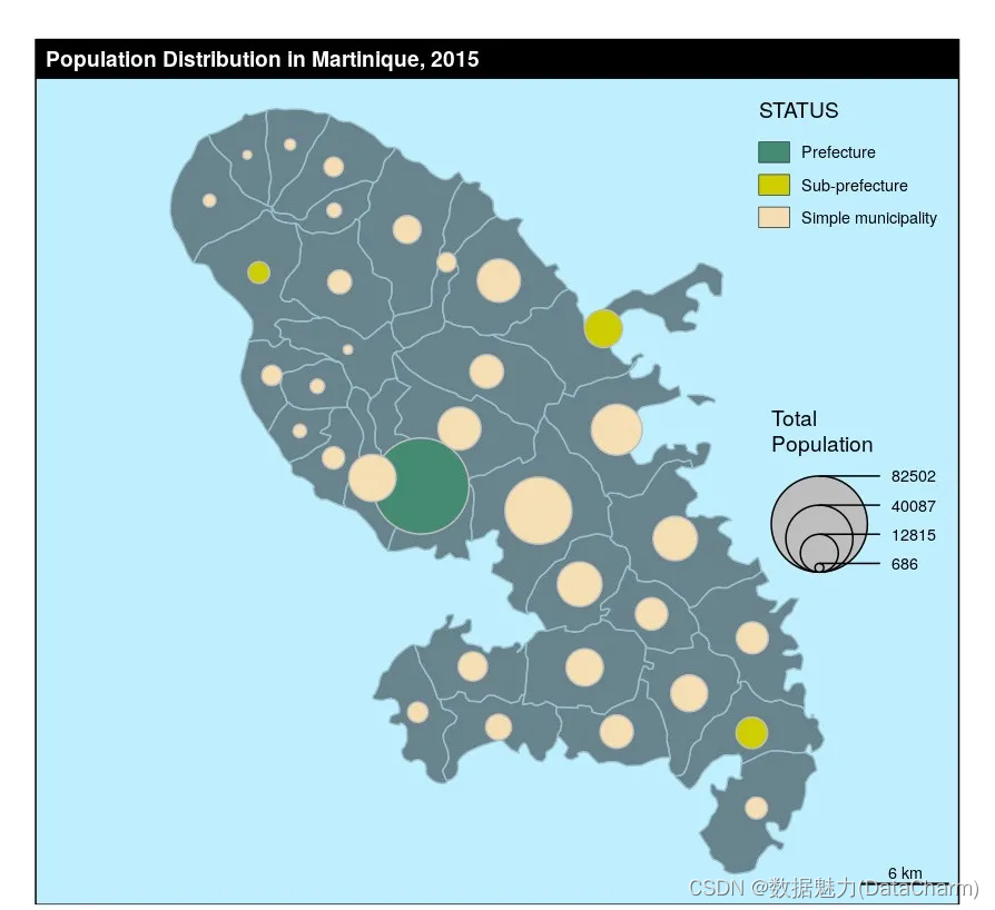
Proportional Symbols Typo Layer

• Double Proportional Triangle Layer

library(sf)
mtq <- st_read(system.file("gpkg/mtq.gpkg", package="cartography"))
mtq$OCC <- mtq$ACT-mtq$CHOM
plot(st_geometry(mtq), col = "lightblue4",border = "lightblue3",
     bg = "lightblue1")
propTrianglesLayer(x = mtq, var1 = "OCC", var2 = "CHOM",
                   col1="green4",col2="red4",k = 0.1)
layoutLayer(title = "Active Population in Martinique, 2015")

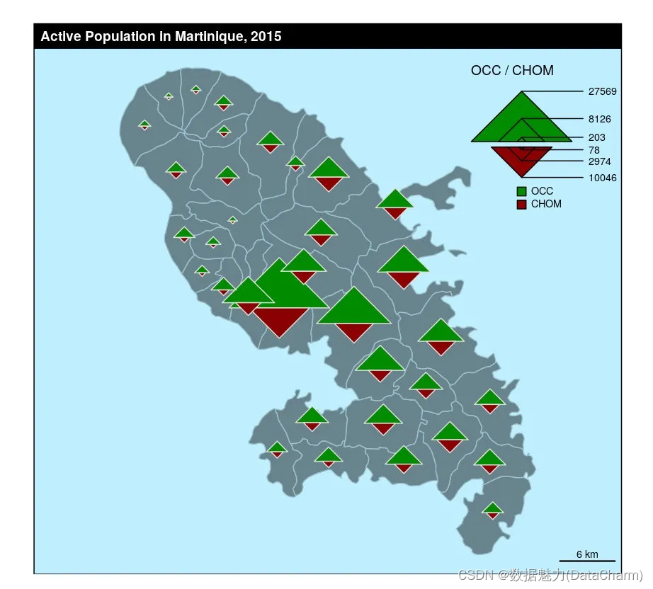
Double Proportional Triangle Layer

• Smooth Layer

library(sf)
mtq <- st_read(system.file("gpkg/mtq.gpkg", package="cartography"))
smoothLayer(x = mtq, var = 'POP',
            span = 4000, beta = 2,
            mask = mtq, border = NA,
            col = carto.pal(pal1 = 'wine.pal', n1 = 8),
            legend.title.txt = "Population\nPotential",
            legend.pos = "topright", legend.values.rnd = 0)
propSymbolsLayer(x = mtq, var = "POP", legend.pos = c(690000, 1599950),
                 legend.title.txt = "Population 2015",
                 col = NA, border = "#ffffff50")
layoutLayer(title = "Actual and Potential Popultation in Martinique")

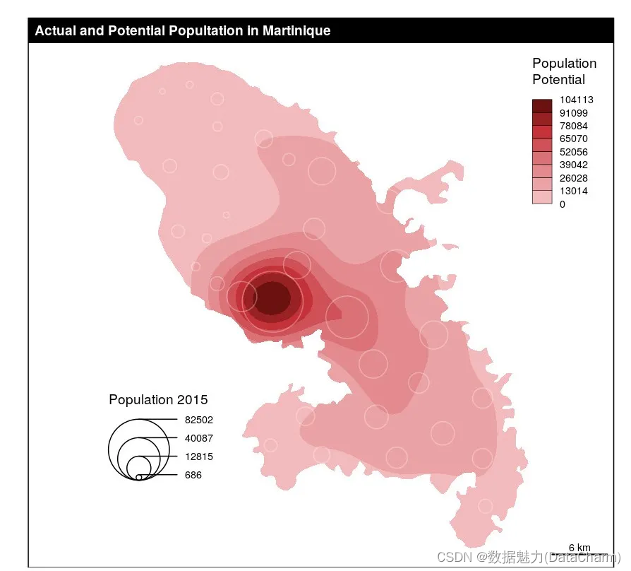
Smooth Layer

• Typology Layer

library(sf)
mtq <- st_read(system.file("gpkg/mtq.gpkg", package="cartography"))
typoLayer(x = mtq, var="STATUS",
          col = c("aquamarine4", "yellow3","wheat"),
          legend.values.order = c("Prefecture",
                                  "Sub-prefecture",
                                  "Simple municipality"),
          legend.pos = "topright",
          legend.title.txt = "Status")
layoutLayer(title = "Municipality Status")

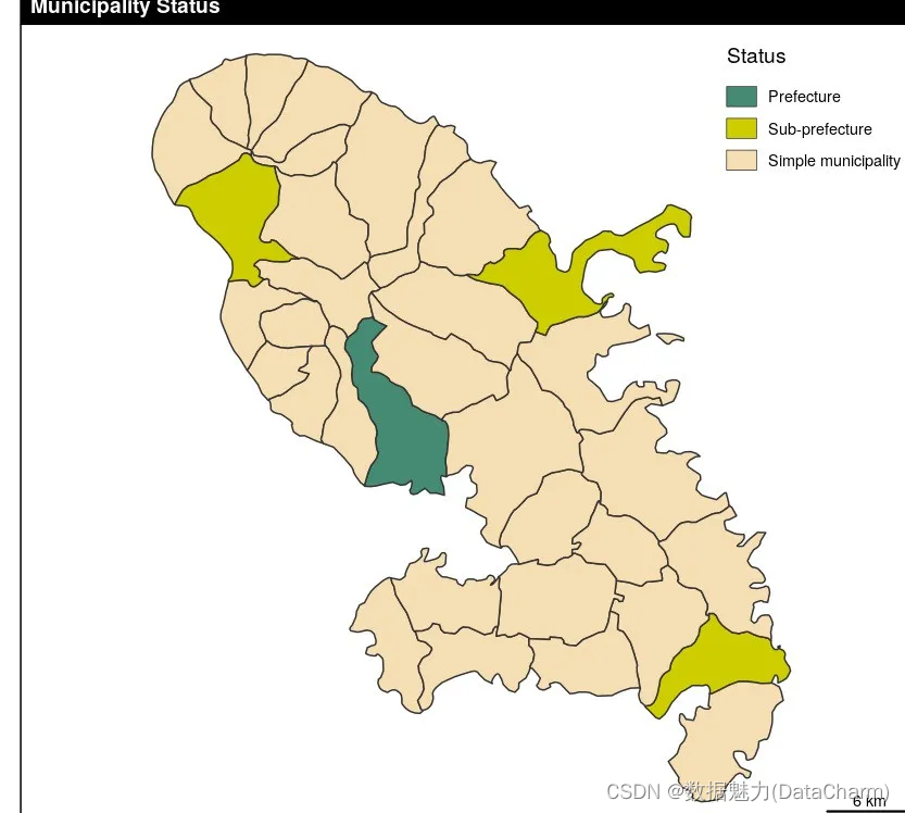
Typology Layer

• Waffle Layer

library(sf)
mtq <- st_read(system.file("gpkg/mtq.gpkg", package = "cartography"),
               quiet = TRUE)
# number of employed persons
mtq$EMP <- mtq$ACT - mtq$CHOM

plot(st_geometry(mtq),
     col = "#f2efe9",
     border = "#b38e43",
     lwd = 0.5)
waffleLayer(
  x = mtq,
  var = c("EMP", "CHOM"),
  cellvalue = 100,
  cellsize = 400,
  cellrnd = "ceiling",
  celltxt = "1 cell represents 100 persons",
  labels = c("Employed", "Unemployed"),
  ncols = 6,
  col = c("tomato1", "lightblue"),
  border = "#f2efe9",
  legend.pos = "topright",
  legend.title.cex = 1,
  legend.title.txt = "Active Population",
  legend.values.cex = 0.8,
  add = TRUE
)

layoutLayer(
  title = "Structure of the Active Population",
  col = "tomato4",
  tabtitle = TRUE,
  scale = FALSE,
  sources =  paste0("cartography ", packageVersion("cartography")),
  author = "Sources: Insee and IGN, 2018",
)

Waffle Layer

• Wordcloud Layer

library(sf)
mtq <- st_read(system.file("gpkg/mtq.gpkg", package = "cartography"))
par(mar=c(0,0,0,0))
plot(st_geometry(mtq),
     col = "white",
     bg = "grey95",
     border = NA)
wordcloudLayer(
  x = mtq,
  txt = "LIBGEO",
  freq = "POP",
  add = TRUE,
  nclass = 5
)
legendChoro(
  title.txt = "Population",
  breaks = getBreaks(mtq$POP, nclass = 5, method = "quantile"),
  col = carto.pal("blue.pal", 5),
  nodata = FALSE
)

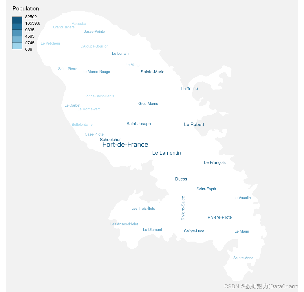
Wordcloud Layer

除此之外，cartography包还提供用于绘制定制化图例的函数，这部分大家可自行探索哈~~

cartography 实例绘制

上面的绘图都来自于cartography官网，接下来，我们使用具体例子进行绘制，使用的数据还是关于美国的。代码如下：

library(sf)
library(cartography)
library(socviz)
library(albersusa)
library(tidyverse)
library(hrbrthemes)

us_sf <- albersusa::usa_sf("laea")
png("usa_03.png",
    units = "in",width = 8,height = 6,res = 600)
# 设置画布边间
par(mar = c(0,0,1.2,0))
plot(st_geometry(us_sf), col = "grey60",border = "white",
     lwd=0.4, bg = "lightsteelblue1")
propSymbolsChoroLayer(x = us_sf, var = "pop_2014", var2 = "census_area",
                      col = carto.pal(pal1 = "blue.pal", n1 = 3,
                                      pal2 = "red.pal", n2 = 3),
                      inches = 0.2, method = "q6",
                      border = "grey50", lwd = 1,
                      legend.var.pos = "topright",
                      legend.var2.pos = "bottomleft",
                      legend.var2.values.rnd = -2,
                      legend.var2.title.txt = "Census Area)",
                      legend.var.title.txt = "Total Population in 2014",
                      legend.var.style = "e")
# First layout
layoutLayer(title="Population and Census Area in USA, 2014",
            author = "Visualization by DataCharm")
# north arrow
north(pos = "topleft")
dev.off()

可视化结果如下：

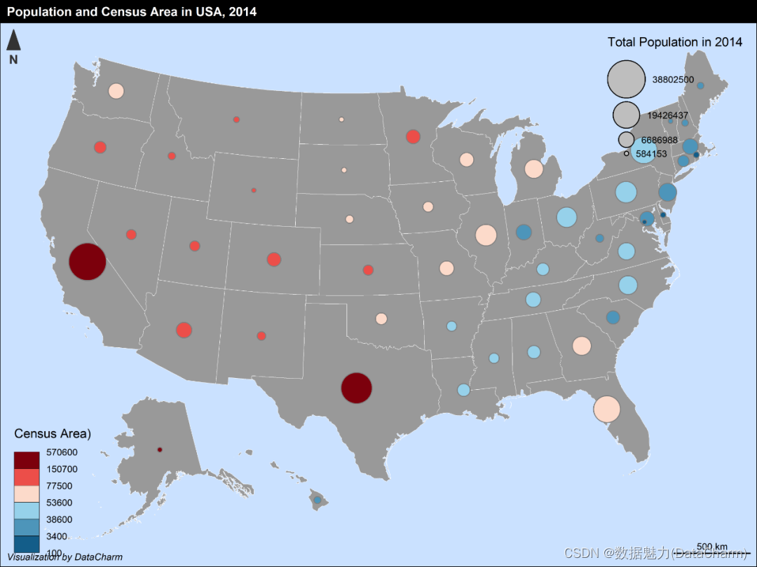
Example Of USA

总结

本期推文我们系统介绍了cartography中常用的地图图层绘制，几乎包括了常见的地图类型，希望小伙伴们可以多多安利这个包~~