【图形学】04 数学部分（四、放射变换）

1、线性变换

线性变换从几何直观有三个要点：

• 变换前是直线的，变换后依然是直线
• 直线比例保持不变
• 变换前是原点的，变换后依然是原点
  比如说旋转，剪切

2、仿射变换

仿射变换从几何直观只有两个要点：

• 变换前是直线的，变换后依然是直线
• 直线比例保持不变

inline Vector2D operator * ( const Vector2D& vec,const Matrix3x3& ma) {
	Vector2D new_vec;
	float x = ma._11 * vec.x + ma._21 * vec.y + ma._31;
	float y = ma._12 * vec.x + ma._22 * vec.y + ma._32;
	float z = ma._13 * vec.x + ma._23 * vec.y + ma._33;
	new_vec.x = x / z;
	new_vec.y = y / z;
	return new_vec;
}

  之前我问过谢老师一个问题，为什么代码第6、7行要除以 z，实际上这就涉及到放射变化的部分，因为平移已经不是。线性变换了，平移之后，原点离开了原来的坐标位置。

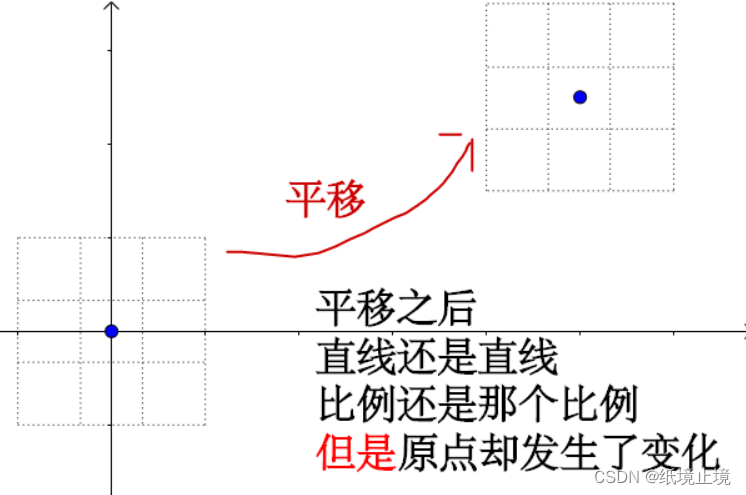
  所以，我们平移的时候，实际上是增加了一个向量[0,0,1]，同时增加了一个维度，最后我们要把我们的向量还原到之前的维度。

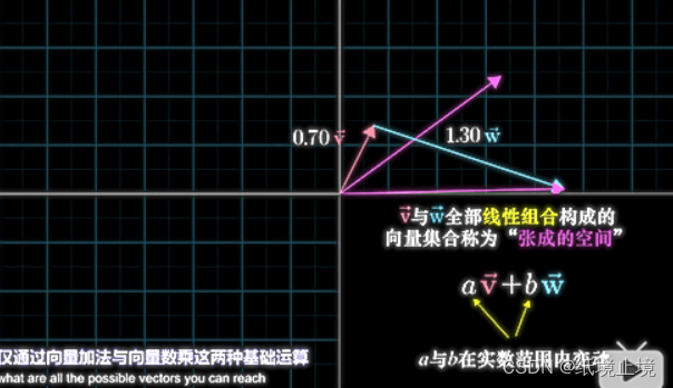
3、张成空间

• 二维的张成空间
  

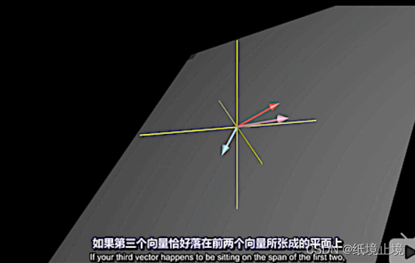
• 三维的张成空间
  

• 线性相关：有多组向量构成张成空间，移除其中一个 不减少 张成空间的大小
  线性无关：所有向量 给张成空间增添了新的维度

• 线性相关：多组向量中，有向量 = 其他向量的线性组合
  

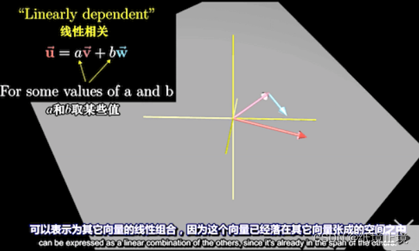
• 齐次向量：表示同一条直线的一类向量

4、对于齐次坐标的理解

参考链接：https://www.cnblogs.com/csyisong/archive/2008/12/09/1351372.html

  “齐次坐标表示是计算机图形学的重要手段之一，它既能够用来明确区分向量和点，同时也更易用于进行仿射（线性）几何变换。”—— F.S. Hill, JR。

  如何在普通坐标(Ordinary Coordinate)和齐次坐标(Homogeneous Coordinate)之间进行转换：

• (1)从普通坐标转换成齐次坐标时
    如果(x,y,z)是个点，则变为(x,y,z,1);
    如果(x,y,z)是个向量，则变为(x,y,z,0)

• (2)从齐次坐标转换成普通坐标时
    如果是(x,y,z,1)，则知道它是个点，变成(x,y,z);
    如果是(x,y,z,0)，则知道它是个向量，仍然变成(x,y,z)

  《GAMES101》中，也介绍了关于3D坐标系下，齐次坐标的问题。

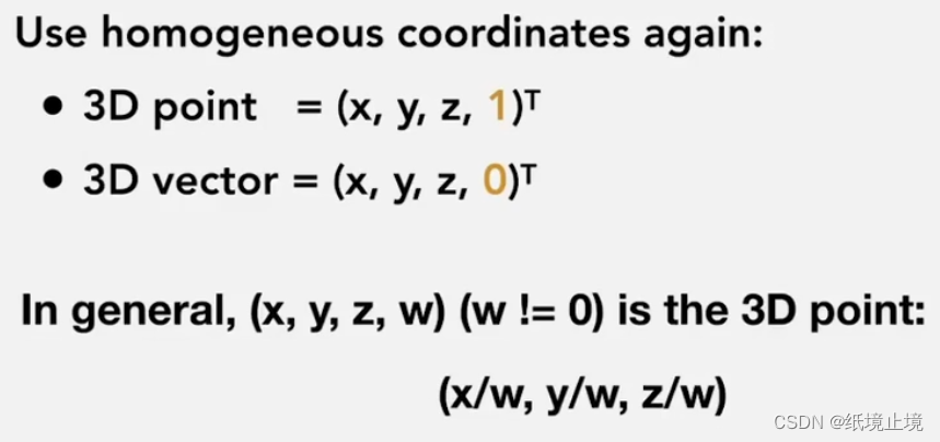
  以上是通过齐次坐标来区分向量和点的方式。从中可以思考得知，对于平移T、旋转R、缩放S这3个最常见的仿射变换，平移变换只对于点才有意义，因为普通向量没有位置概念，只有大小和方向。
  而旋转和缩放对于向量和点都有意义，你可以用类似上面齐次表示来检测。从中可以看出，齐次坐标用于仿射变换非常方便。

  此外，对于一个普通坐标的点P=(Px, Py, Pz)，有对应的一族齐次坐标(wPx, wPy, wPz, w)，其中w不等于零。比如，P(1, 4, 7)的齐次坐标有(1, 4, 7, 1)、（2, 8, 14, 2）、（-0.1, -0.4, -0.7, -0.1）等等。因此，如果把一个点从普通坐标变成齐次坐标，给x,y,z乘上同一个非零数w，然后增加第4个分量w；如果把一个齐次坐标转换成普通坐标，把前三个坐标同时除以第4个坐标，然后去掉第4个分量。

  由于齐次坐标使用了4个分量来表达3D概念，使得平移变换可以使用矩阵进行，从而如F.S. Hill, JR所说，仿射（线性）变换的进行更加方便。由于图形硬件已经普遍地支持齐次坐标与矩阵乘法，因此更加促进了齐次坐标使用，使得它似乎成为图形学中的一个标准。

n、多边形重心的推论

Yes, yes, but why? The current answers (as well as Wikipedia) do not contain enough detail to understand these formulas immediately. So let’s start with the very basic definition of the area centroid: $$\vec{C}=\frac{\iint \vec{r}(x,y)dxdy}{\iint dxdy}=\frac{(\iint xdxdy,\iint ydxdy)}{\iint dxdy}=\frac{(m_x,m_y)}{A}=(C_x,C_y)$$ Allright, let’s get rid of the double integrals in the first place, by employing Green’s theorem : $$\iint \left(\frac{\partial M}{\partial x}-\frac{\partial L}{\partial y}\right)dxdy=\oint \left(Ldx+Mdy\right)$$ At the edges of the (convex) polygon we have: KaTeX parse error: Undefined control sequence: \mbox at position 88: …d{cases} \quad \̲m̲b̲o̲x̲{with} \quad \b… Then by substitution of $M(x,y)=x$ and $L(x,y)=0$ we have: $$\begin{gathered} A=\iint dxdy=\oint xdy=\sum _{i=0}^{n-1}{\int }_0^1\left[x_i+(x_{i+}-x_i)t\right](y_{i+}-y_i)dt= \\ \sum _{i=0}^{n-1}(y_{i+}-y_i)\left[x_i{t|}_0^1+(x_{i+}-x_i)\frac{1}{2}{t^2|}_0^1\right]=\frac{1}{2}\sum _{i=0}^{n-1}(x_{i+}+x_i)(y_{i+}-y_i)= \\ \frac{1}{2}\sum _{i=0}^{n-1}(x_i{y}_{i+}-x_{i+}{y}_i) \end{gathered}$$ The last move by telescoping.
The main integral for the $x$-coordinate of the centroid is,
with $M(x,y)=x^2/2$ and $L(x,y)=0$: $$\begin{gathered} m_x=\iint xdxdy=\oint \frac{1}{2}{x}^{2}dy=\frac{1}{2}\sum _{i=0}^{n-1}(y_{i+}-y_i){\int }_0^1{\left[x_i+(x_{i+}-x_i)t\right]}^{2}dt= \\ \frac{1}{2}\sum _{i=0}^{n-1}(y_{i+}-y_i)\left[x_i^2{t|}_0^1+2x_i(x_{i+}-x_i)\frac{1}{2}{t^2|}_0^1+(x_{i+}-x_i{)}^2\frac{1}{3}{t^3|}_0^1\right]= \\ \frac{1}{2}\sum _{i=0}^{n-1}(y_{i+}-y_i)\left[x_i^2+x_i(x_{i+}-x_i)+\frac{1}{3}(x_{i+}-x_i{)}^2\right]= \\ \frac{1}{6}\sum _{i=0}^{n-1}(y_{i+}-y_i)\left[x_{i+}^2+x_i{x}_{i+}+x_i^2\right]= \\ \frac{1}{6}\sum _{i=0}^{n-1}\left[x_i{x}_{i+}{y}_{i+}+x_i^2{y}_{i+}-x_{i+}^2{y}_i-x_i{x}_{i+}{y}_i\right]⟹ \\ {m}_x=\frac{1}{6}\sum _{i=0}^{n-1}(x_i+x_{i+})(x_i{y}_{i+}-x_{i+}{y}_i) \end{gathered}$$ The last two moves after telescoping again.
The main integral for the $y$-coordinate of the area centroid is,
with $M(x,y)=0$ and $L(x,y)=-y^2/2$: $$m_y=\iint ydxdy=\oint -\frac{1}{2}{y}^{2}dx=-\frac{1}{2}\sum _{i=0}^{n-1}(x_{i+}-x_i){\int }_0^1{\left[y_i+(y_{i+}-y_i)t\right]}^{2}dt$$ Which is similar to the main integral for the $x$-coordinate of the centroid: $$m_x=\iint xdxdy=\oint \frac{1}{2}{x}^{2}dy=\frac{1}{2}\sum _{i=0}^{n-1}(y_{i+}-y_i){\int }_0^1{\left[x_i+(x_{i+}-x_i)t\right]}^{2}dt$$ It is seen that everything is the same if we just exchange $x$ and $y$, except for the minus sign, hence: $$m_y=-\frac{1}{6}\sum _{i=0}^{n-1}(y_i+y_{i+})(y_i{x}_{i+}-y_{i+}{x}_i)=\frac{1}{6}\sum _{i=0}^{n-1}(y_i+y_{i+})(x_i{y}_{i+}-x_{i+}{y}_i)$$ Combining the partial results found gives the end result, as displayed in the question.