十、评估指标

我看过很多课程，不过内容都大差不差，也可以参考这篇模型评估方法

一、K折交叉验证

一般情况，我们得到一份数据集，会分为两类，一类是trainset训练集，另一类十testset测试集。通俗一点也就是训练集相当于平常的练习册，直接去刷题；测试集就是高考，只有一次！而且还没见过。但是一味的刷题真的好吗？

这时，交叉验证(Cross-validation)出现了，也成为CV，啥意思呢？就是将训练集再进行划分为trainset训练集和validset验证集，验证集去充当期末考试，这是不是就合理多了。
例如：1000份数据，原本是200测试集、800训练集；当交叉验证引进之后就变成了200测试集、600训练集、200验证集。这里的验证集是从原本的训练集中来的。
800训练集，通过交叉验证分为了600训练集、200验证集，也就是分成了四份，这就是四折交叉验证。同理将训练集分成几份就是几折交叉验证。一般情况验证集占一份即可。

交叉验证(Cross-validation)主要应用于建模中，例如PCR、PLS回归建模，在给定的建模样本中，留出一小部分，用刚训练出来的模型进行预测，并求出这小部分的样本预测误差，记录一下平方加和。

实时上，模型中有很多的超参数需要用户进行传入，不单单是学习率α一个，还有收敛阈值、泛化能力值等，这时候咋办捏？GridSearchCV来了！

二、GridSearchCV

这玩意儿其实就是个函数，很厉害啊，别小看人家。它可以将你传入的多个超参数进行排列组合，然后代入模型中进行训练，最后返回出效果最佳的超参数。这就不需要人为的去傻了吧唧的一个一个的调参选出最优解了。
GridSearchCV(log_reg, param_grid=param_grid, cv=3)
第一个参数：要对哪一个模型进行训练
第二个参数：选择的超参数有哪些
第三个参数：几折交叉验证

三、代码实战

import numpy as np
from sklearn import datasets
from sklearn.linear_model import LogisticRegression
from sklearn.model_selection import GridSearchCV
import matplotlib.pyplot as plt
from time import time

iris = datasets.load_iris()
#print(list(iris.keys()))
#print(iris['DESCR'])
#print(iris['feature_names'])#特征名

X = iris['data'][:, 3:]#取出x矩阵
#print(X)#petal width(cm)

#print(iris['target'])
y = iris['target']
# y = (iris['target'] == 2).astype(np.int)
#print(y)#获取类别号


# Utility function to report best scores
def report(results, n_top=3):
    for i in range(1, n_top + 1):
        candidates = np.flatnonzero(results['rank_test_score'] == i)
        for candidate in candidates:
            print("Model with rank: {0}".format(i))
            print("Mean validation score: {0:.3f} (std: {1:.3f})".format(
                  results['mean_test_score'][candidate],
                  results['std_test_score'][candidate]))
            print("Parameters: {0}".format(results['params'][candidate]))
            print("")


start = time()
# tol收敛的阈值超参数
# C泛化能力，越小泛化能力越高
param_grid = {"tol": [1e-4, 1e-3, 1e-2],
              "C": [0.4, 0.6, 0.8]}
log_reg = LogisticRegression(multi_class='ovr', solver='sag')#多个二分类来解决多分类为ovr，若为multinomial则使用softmax求解多分类问题；梯度下降法sag；
grid_search = GridSearchCV(log_reg, param_grid=param_grid, cv=3)
"""
GridSearchCV函数
第一个参数：要对哪一个模型进行训练
第二个参数：选择的超参数有哪些
第三个参数：几折交叉验证
"""
grid_search.fit(X, y)
print("GridSearchCV took %.2f seconds for %d candidate parameter settings."
      % (time() - start, len(grid_search.cv_results_['params'])))
report(grid_search.cv_results_)


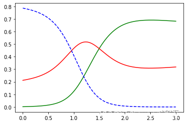
X_new = np.linspace(0, 3, 1000).reshape(-1, 1)#创建新的数据集，从0-3这个区间范围内，取1000个数值，linspace为平均分成1000个段，取出1000个点
#print(X_new)

y_proba = grid_search.predict_proba(X_new)#预测分类号具体分类成哪一个类别的概率值
y_hat = grid_search.predict(X_new)#预测分类号具体分类成哪一个类别，跟0.5去比较，从而划分为0或者1
print(y_proba)
print(y_hat)
print("w1",grid_search.best_estimator_)


plt.plot(X_new, y_proba[:, 2], 'g-', label='Iris-Virginica')
plt.plot(X_new, y_proba[:, 1], 'r-', label='Iris-Versicolour')
plt.plot(X_new, y_proba[:, 0], 'b--', label='Iris-Setosa')
plt.show()

print(grid_search.predict([[1.7], [1.5]]))
"""
GridSearchCV took 0.05 seconds for 9 candidate parameter settings.
Model with rank: 1
Mean validation score: 0.907 (std: 0.025)
Parameters: {'C': 0.6, 'tol': 0.0001}

Model with rank: 1
Mean validation score: 0.907 (std: 0.025)
Parameters: {'C': 0.6, 'tol': 0.001}

Model with rank: 1
Mean validation score: 0.907 (std: 0.025)
Parameters: {'C': 0.6, 'tol': 0.01}

Model with rank: 1
Mean validation score: 0.907 (std: 0.025)
Parameters: {'C': 0.8, 'tol': 0.0001}

Model with rank: 1
Mean validation score: 0.907 (std: 0.025)
Parameters: {'C': 0.8, 'tol': 0.001}

Model with rank: 1
Mean validation score: 0.907 (std: 0.025)
Parameters: {'C': 0.8, 'tol': 0.01}

[[7.85881224e-01 2.11932164e-01 2.18661232e-03]
 [7.85645909e-01 2.12143369e-01 2.21072210e-03]
 [7.85409133e-01 2.12355759e-01 2.23510765e-03]
 ...
 [1.25568737e-04 3.17858272e-01 6.82016160e-01]
 [1.24101822e-04 3.17945561e-01 6.81930337e-01]
 [1.22652125e-04 3.18033028e-01 6.81844320e-01]]
[0 0 0 0 0 0 0 0 0 0 0 0 0 0 0 0 0 0 0 0 0 0 0 0 0 0 0 0 0 0 0 0 0 0 0 0 0
 0 0 0 0 0 0 0 0 0 0 0 0 0 0 0 0 0 0 0 0 0 0 0 0 0 0 0 0 0 0 0 0 0 0 0 0 0
 0 0 0 0 0 0 0 0 0 0 0 0 0 0 0 0 0 0 0 0 0 0 0 0 0 0 0 0 0 0 0 0 0 0 0 0 0
 0 0 0 0 0 0 0 0 0 0 0 0 0 0 0 0 0 0 0 0 0 0 0 0 0 0 0 0 0 0 0 0 0 0 0 0 0
 0 0 0 0 0 0 0 0 0 0 0 0 0 0 0 0 0 0 0 0 0 0 0 0 0 0 0 0 0 0 0 0 0 0 0 0 0
 0 0 0 0 0 0 0 0 0 0 0 0 0 0 0 0 0 0 0 0 0 0 0 0 0 0 0 0 0 0 0 0 0 0 0 0 0
 0 0 0 0 0 0 0 0 0 0 0 0 0 0 0 0 0 0 0 0 0 0 0 0 0 0 0 0 0 0 0 0 0 0 0 0 0
 0 0 0 0 0 0 0 0 0 0 0 0 0 0 0 0 0 0 0 0 0 0 0 0 0 0 0 0 0 0 0 0 0 0 0 0 0
 0 0 0 0 0 0 0 0 0 0 0 0 0 0 0 0 0 0 0 0 0 0 1 1 1 1 1 1 1 1 1 1 1 1 1 1 1
 1 1 1 1 1 1 1 1 1 1 1 1 1 1 1 1 1 1 1 1 1 1 1 1 1 1 1 1 1 1 1 1 1 1 1 1 1
 1 1 1 1 1 1 1 1 1 1 1 1 1 1 1 1 1 1 1 1 1 1 1 1 1 1 1 1 1 1 1 1 1 1 1 1 1
 1 1 1 1 1 1 1 1 1 1 1 1 1 1 1 1 1 1 1 1 1 1 1 1 1 1 1 1 1 1 1 1 1 1 1 1 1
 1 1 1 1 1 1 1 1 1 1 1 1 1 1 1 1 1 1 1 1 1 1 1 1 1 1 1 1 1 1 1 1 1 1 1 1 1
 1 1 1 1 1 1 1 1 1 1 1 1 1 1 1 1 1 1 2 2 2 2 2 2 2 2 2 2 2 2 2 2 2 2 2 2 2
 2 2 2 2 2 2 2 2 2 2 2 2 2 2 2 2 2 2 2 2 2 2 2 2 2 2 2 2 2 2 2 2 2 2 2 2 2
 2 2 2 2 2 2 2 2 2 2 2 2 2 2 2 2 2 2 2 2 2 2 2 2 2 2 2 2 2 2 2 2 2 2 2 2 2
 2 2 2 2 2 2 2 2 2 2 2 2 2 2 2 2 2 2 2 2 2 2 2 2 2 2 2 2 2 2 2 2 2 2 2 2 2
 2 2 2 2 2 2 2 2 2 2 2 2 2 2 2 2 2 2 2 2 2 2 2 2 2 2 2 2 2 2 2 2 2 2 2 2 2
 2 2 2 2 2 2 2 2 2 2 2 2 2 2 2 2 2 2 2 2 2 2 2 2 2 2 2 2 2 2 2 2 2 2 2 2 2
 2 2 2 2 2 2 2 2 2 2 2 2 2 2 2 2 2 2 2 2 2 2 2 2 2 2 2 2 2 2 2 2 2 2 2 2 2
 2 2 2 2 2 2 2 2 2 2 2 2 2 2 2 2 2 2 2 2 2 2 2 2 2 2 2 2 2 2 2 2 2 2 2 2 2
 2 2 2 2 2 2 2 2 2 2 2 2 2 2 2 2 2 2 2 2 2 2 2 2 2 2 2 2 2 2 2 2 2 2 2 2 2
 2 2 2 2 2 2 2 2 2 2 2 2 2 2 2 2 2 2 2 2 2 2 2 2 2 2 2 2 2 2 2 2 2 2 2 2 2
 2 2 2 2 2 2 2 2 2 2 2 2 2 2 2 2 2 2 2 2 2 2 2 2 2 2 2 2 2 2 2 2 2 2 2 2 2
 2 2 2 2 2 2 2 2 2 2 2 2 2 2 2 2 2 2 2 2 2 2 2 2 2 2 2 2 2 2 2 2 2 2 2 2 2
 2 2 2 2 2 2 2 2 2 2 2 2 2 2 2 2 2 2 2 2 2 2 2 2 2 2 2 2 2 2 2 2 2 2 2 2 2
 2 2 2 2 2 2 2 2 2 2 2 2 2 2 2 2 2 2 2 2 2 2 2 2 2 2 2 2 2 2 2 2 2 2 2 2 2
 2]
w1 LogisticRegression(C=0.6, multi_class='ovr', solver='sag')
"""

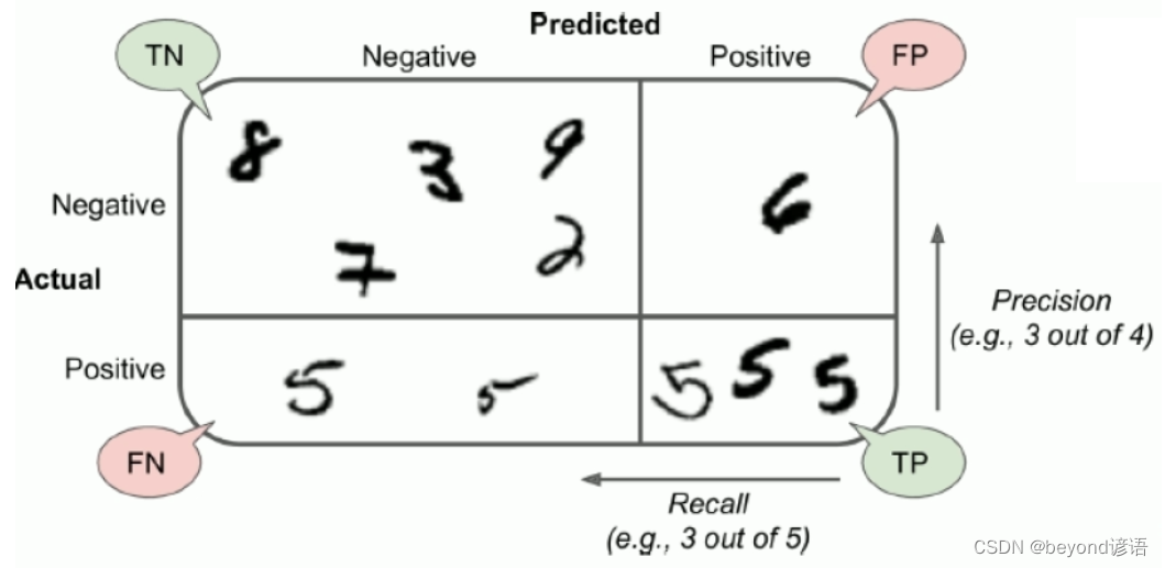
四、混淆矩阵

以MNIST手写数字识别数据集为例，其对于的混淆矩阵如图：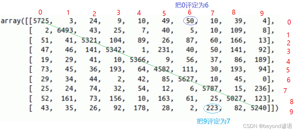
当然，对角线上的数值比较大，也就是判断正确样本数

五、准确率、召回率

P：你认为的是正例
N：你认为的是负例
例如：你要找全班的女生，此时男生就成为了负例，相应的女生就成为了正例。
T：判断正确
F：判断错误
判断正确很好理解，人家是男生，你判断成为了男生，那就是T；你判断成了女生，那就是F。
TP：你认为是正例(P)，最后实际上这个就是正例，判断正确(T)。一个人，你觉得人家是女生，实际上人家就是个女生，判断正确，这就是TP。
FP：你认为是正例(P)，最后实际上这个却是负例，判断错误(F)。一个人，你觉得人家是女生，但实际上人家是个男生，判断错误，这就是FP。
TN：你认为是负例(N)，最后实际上这个就是负例，判断正确(T)。一个人，你觉得人家是男生，实际上人家就是个男生，判断正确，这就是TN。
FN：你认为是负例(N)，最后实际上这个却是负例，判断错误(T)。一个人，你觉得人家是男生，但实际上人家是个女生，判断错误，这就是FN。

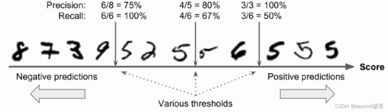
Ⅰ，准确率

准确率：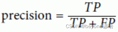
准确率更看重正例的表现
准确率就是在你认为是正确的样例中，真正判断对的有多少
例如：某购物软件给二狗子推荐了10种商品(系统认为这是二狗子喜欢的东西)，但二狗子就选了3个点(实际上二狗子真正喜欢的东西)进去看了看。此时的准确率就是3/10=30%
随着系统推荐的商品越来越多，准确率是下降的，因为分母是在变大。这就相当于言多必失！

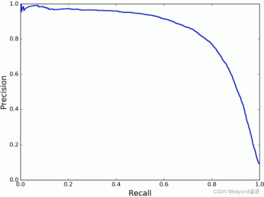
Ⅱ，召回率

召回率：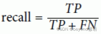
召回率也就是从真正正确的样例中，召回了多少
例如：某购物软件给二狗子推荐了10种商品(系统认为这是二狗子喜欢的东西)，但二狗子就选了3个点(实际上二狗子真正喜欢的东西)进去看了看，二狗子实际上真正喜欢1000种商品(真正的正确样例)，也就是系统仅仅从二狗子喜欢的1000种商品中推选了3个给他。此时的召回率就是3/1000=0.3%
随着系统推荐的商品越来越多，召回率是上升的，因为用户喜欢的商品的总数是不变的，分母不变，推荐的越多越容易出现用户喜欢的商品，也就是分子会越大。

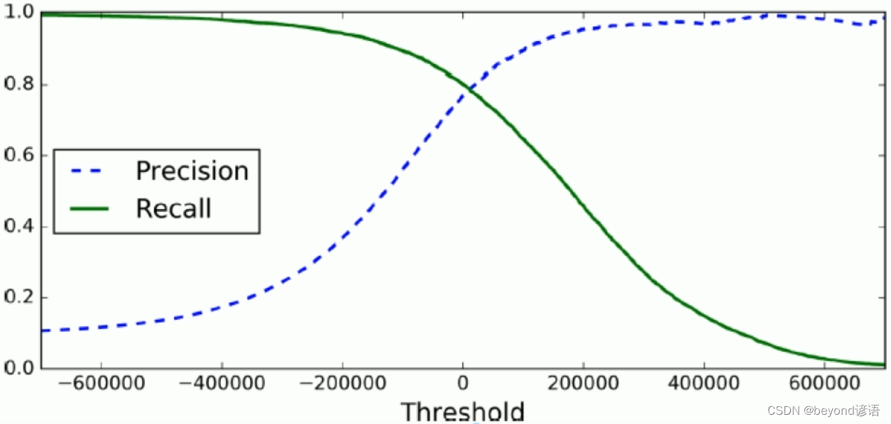
很显然，准确率和召回率是相互抑制的关系，根据需要选择其中一个指标作为核心，进行着重优化考虑，鱼和熊掌不可兼得。
例如：给未成年人推荐视频，宁可拒绝很多好的视频，也不能推荐一个不良视频，此时，就得使用低召回率，也就是要提高准确率。
监控画面抓小偷，宁可把很多人都设成嫌疑犯，宁可工作量大一点，也不能错过一个，也就是所谓的宁可错杀一千也不放过一个，此时就需要高召回率，也就是要低准确率。

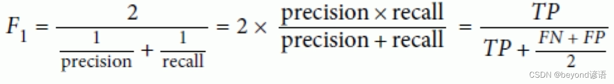
六、F1-Score(F1-Measure)

一个模型的好坏，单从准确率或者召回率看很显然是不够全面的，此时就出现了F1-Score，也称F1-Measure。

七、TradeOff

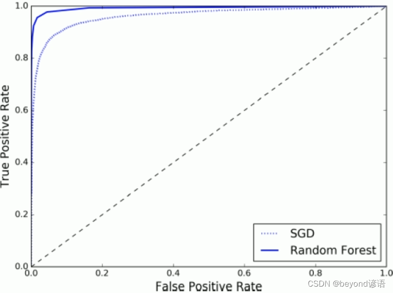
八、ROC曲线(Receiver Characteristic Operator)

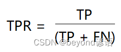，即所有正例中被正确的判定为正例的比例
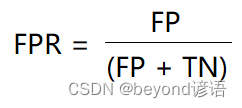，即所有负例中被错误的评定为正例的比例

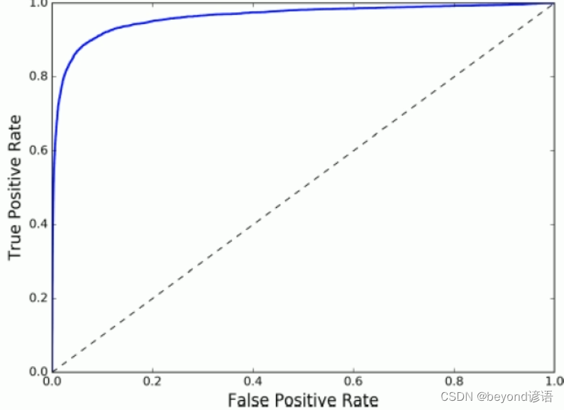
九、AUC面积(Area under Curve曲线下面积)

十、代码实现

from sklearn.datasets import fetch_mldata
import matplotlib
import matplotlib.pyplot as plt
import numpy as np
from sklearn.linear_model import SGDClassifier
from sklearn.model_selection import StratifiedKFold
from sklearn.base import clone
from sklearn.model_selection import cross_val_score
from sklearn.base import BaseEstimator
from sklearn.model_selection import cross_val_predict
from sklearn.metrics import confusion_matrix
from sklearn.metrics import precision_score
from sklearn.metrics import recall_score
from sklearn.metrics import f1_score
from sklearn.metrics import precision_recall_curve
from sklearn.metrics import roc_curve
from sklearn.metrics import roc_auc_score
from sklearn.ensemble import RandomForestClassifier


mnist = fetch_mldata('MNIST original', data_home='test_data_home')
print(mnist)
"""
{'DESCR': 'mldata.org dataset: mnist-original', 'COL_NAMES': ['label', 'data'], 'target': array([0., 0., 0., ..., 9., 9., 9.]), 'data': array([[0, 0, 0, ..., 0, 0, 0],
       [0, 0, 0, ..., 0, 0, 0],
       [0, 0, 0, ..., 0, 0, 0],
       ...,
       [0, 0, 0, ..., 0, 0, 0],
       [0, 0, 0, ..., 0, 0, 0],
       [0, 0, 0, ..., 0, 0, 0]], dtype=uint8)}
"""

X, y = mnist['data'], mnist['target']
print(X.shape, y.shape)
"""
(70000, 784) (70000,)
"""

some_digit = X[36000]
print(some_digit)
some_digit_image = some_digit.reshape(28,28)
print(some_digit_image)

#?(28,28)???????
# plt.imshow(some_digit_image, cmap=matplotlib.cm.binary,
#            interpolation='nearest')
# plt.axis('off')
# plt.show()

#??60000??????????
X_train, X_test, y_train, y_test = X[:60000], X[60000:], y[:60000], y[:60000]
shuffle_index = np.random.permutation(60000)
X_train, y_train = X_train[shuffle_index], y_train[shuffle_index]

y_train_5 = (y_train == 5)
y_test_5 = (y_test == 5)
print(y_test_5)
"""
[False False False ... False False False]
"""


sgd_clf = SGDClassifier(loss='log', random_state=42,max_iter=500)
sgd_clf.fit(X_train, y_train_5)
print(sgd_clf.predict([some_digit]))
"""
[ True]
"""



# skfolds = StratifiedKFold(n_splits=3, random_state=42)
#
# for train_index, test_index in skfolds.split(X_train, y_train_5):
#     clone_clf = clone(sgd_clf)
#     X_train_folds = X_train[train_index]
#     y_train_folds = y_train_5[train_index]
#     X_test_folds = X_train[test_index]
#     y_test_folds = y_train_5[test_index]
#
#     clone_clf.fit(X_train_folds, y_train_folds)
#     y_pred = clone_clf.predict(X_test_folds)
#     print(y_pred)
#     n_correct = sum(y_pred == y_test_folds)
#     print(n_correct / len(y_pred))

'''
print(cross_val_score(sgd_clf, X_train, y_train_5, cv=3, scoring='accuracy'))
"""
[0.91185 0.95395 0.9641 ]
"""
print(cross_val_score(sgd_clf, X_train, y_train_5, cv=3, scoring='precision'))
"""
[0.50661455 0.69741533 0.81972989]
"""
'''


# class Never5Classifier(BaseEstimator):
#     def fit(self, X, y=None):
#         pass
#
#     def predict(self, X):
#         return np.zeros((len(X), 1), dtype=bool)
#
#
# never_5_clf = Never5Classifier()
# print(cross_val_score(never_5_clf, X_train, y_train_5, cv=3, scoring='accuracy'))
# """
# [0.9098  0.9094  0.90975]
# """


y_train_pred = cross_val_predict(sgd_clf, X_train, y_train_5, cv=3)
print(confusion_matrix(y_train_5, y_train_pred))
"""
[[53553  1026]
 [ 1737  3684]]
"""

y_train_perfect_prediction = y_train_5
print(confusion_matrix(y_train_5, y_train_perfect_prediction))
"""
[[54579     0]
 [    0  5421]]
"""

print(precision_score(y_train_5, y_train_pred))
print(recall_score(y_train_5, y_train_pred))
print(sum(y_train_pred))
print(f1_score(y_train_5, y_train_pred))
"""
0.7821656050955414
0.679579413392363
4710
0.7272727272727272
"""



sgd_clf.fit(X_train, y_train_5)
y_scores = sgd_clf.decision_function([some_digit])
print(y_scores)

threshold = 0
y_some_digit_pred = (y_scores > threshold)
print(y_some_digit_pred)

threshold = 200000
y_some_digit_pred = (y_scores > threshold)
print(y_some_digit_pred)

y_scores = cross_val_predict(sgd_clf, X_train, y_train_5, cv=3, method='decision_function')
print(y_scores)

precisions, recalls, thresholds = precision_recall_curve(y_train_5, y_scores)
print(precisions, recalls, thresholds)


def plot_precision_recall_vs_threshold(precisions, recalls, thresholds):
    plt.plot(thresholds, precisions[:-1], 'b--', label='Precision')
    plt.plot(thresholds, recalls[:-1], 'r--', label='Recall')
    plt.xlabel("Threshold")
    plt.legend(loc='upper left')
    plt.ylim([0, 1])


plot_precision_recall_vs_threshold(precisions, recalls, thresholds)
plt.show()


y_train_pred_90 = (y_scores > 70000)
print(precision_score(y_train_5, y_train_pred_90))
print(recall_score(y_train_5, y_train_pred_90))


fpr, tpr, thresholds = roc_curve(y_train_5, y_scores)


def plot_roc_curve(fpr, tpr, label=None):
    plt.plot(fpr, tpr, linewidth=2, label=label)
    plt.plot([0, 1], [0, 1], 'k--')
    plt.axis([0, 1, 0, 1])
    plt.xlabel('False Positive Rate')
    plt.ylabel('True positive Rate')


plot_roc_curve(fpr, tpr)
plt.show()

print(roc_auc_score(y_train_5, y_scores))

forest_clf = RandomForestClassifier(random_state=42)
y_probas_forest = cross_val_predict(forest_clf, X_train, y_train_5, cv=3, method='predict_proba')
y_scores_forest = y_probas_forest[:, 1]

fpr_forest, tpr_forest, thresholds_forest = roc_curve(y_train_5, y_scores_forest)
plt.plot(fpr, tpr, 'b:', label='SGD')
plt.plot(fpr_forest, tpr_forest, label='Random Forest')
plt.legend(loc='lower right')
plt.show()

print(roc_auc_score(y_train_5, y_scores_forest))