


概述:
本篇博文,使用逻辑回归进行银行卡欺诈分析,对于不均衡样本的数据预处理处理展示了两种方法:
- 向下采样策略
- 向上采样策略(文中使用SMOTE算法)
然后对比了数据进行上述处理前后的效果对比。此外还对不同阈值对分类模型的影响进行了探讨。文中有完整的代码和图示。并有详细的中英文代码注释。
涉及到的技术有:
- pandas库
- numpy库
- sklearn库
- imblearn库
- matplot库
下面是正文:
import pandas as pd
import matplotlib.pyplot as plt
import numpy as np

%matplotlib inline
data = pd.read_csv("creditcard.csv")
data.head()
| Time | V1 | V2 | V3 | V4 | V5 | V6 | V7 | V8 | V9 | ... | V21 | V22 | V23 | V24 | V25 | V26 | V27 | V28 | Amount | Class | |
|---|---|---|---|---|---|---|---|---|---|---|---|---|---|---|---|---|---|---|---|---|---|
| 0 | 0.0 | -1.359807 | -0.072781 | 2.536347 | 1.378155 | -0.338321 | 0.462388 | 0.239599 | 0.098698 | 0.363787 | ... | -0.018307 | 0.277838 | -0.110474 | 0.066928 | 0.128539 | -0.189115 | 0.133558 | -0.021053 | 149.62 | 0 |
| 1 | 0.0 | 1.191857 | 0.266151 | 0.166480 | 0.448154 | 0.060018 | -0.082361 | -0.078803 | 0.085102 | -0.255425 | ... | -0.225775 | -0.638672 | 0.101288 | -0.339846 | 0.167170 | 0.125895 | -0.008983 | 0.014724 | 2.69 | 0 |
| 2 | 1.0 | -1.358354 | -1.340163 | 1.773209 | 0.379780 | -0.503198 | 1.800499 | 0.791461 | 0.247676 | -1.514654 | ... | 0.247998 | 0.771679 | 0.909412 | -0.689281 | -0.327642 | -0.139097 | -0.055353 | -0.059752 | 378.66 | 0 |
| 3 | 1.0 | -0.966272 | -0.185226 | 1.792993 | -0.863291 | -0.010309 | 1.247203 | 0.237609 | 0.377436 | -1.387024 | ... | -0.108300 | 0.005274 | -0.190321 | -1.175575 | 0.647376 | -0.221929 | 0.062723 | 0.061458 | 123.50 | 0 |
| 4 | 2.0 | -1.158233 | 0.877737 | 1.548718 | 0.403034 | -0.407193 | 0.095921 | 0.592941 | -0.270533 | 0.817739 | ... | -0.009431 | 0.798278 | -0.137458 | 0.141267 | -0.206010 | 0.502292 | 0.219422 | 0.215153 | 69.99 | 0 |
5 rows × 31 columns
#count_classes = pd.value_counts(data['Class'], sort = True).sort_index() #
#把某列数据传入,自动计算各类型数据的数量
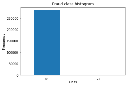
count_classes = pd.value_counts(data['Class'], sort = True)
count_classes.plot(kind = 'bar')
plt.title("Fraud class histogram")
plt.xlabel("Class")
plt.ylabel("Frequency")
Text(0, 0.5, 'Frequency')
#sklearn(库)中有数据预处理模块(processing) and 函数(StandardScaler)
from sklearn.preprocessing import StandardScaler

# 将给定数据进行标准化,并作为新的一列存入data(新的列名“normAmount”)
# data['normAmount'] = StandardScaler().fit_transform(data['Amount'].reshape(-1, 1)) #已弃用,原因,data[]的类型是series,而data[].values类型是numpy.ndarray which support reshape operation
data['normAmount'] = StandardScaler().fit_transform(data['Amount'].values.reshape(-1,1))

# 丢弃指定的列
data = data.drop(['Time','Amount'],axis=1)
data.head()
| V1 | V2 | V3 | V4 | V5 | V6 | V7 | V8 | V9 | V10 | ... | V21 | V22 | V23 | V24 | V25 | V26 | V27 | V28 | Class | normAmount | |
|---|---|---|---|---|---|---|---|---|---|---|---|---|---|---|---|---|---|---|---|---|---|
| 0 | -1.359807 | -0.072781 | 2.536347 | 1.378155 | -0.338321 | 0.462388 | 0.239599 | 0.098698 | 0.363787 | 0.090794 | ... | -0.018307 | 0.277838 | -0.110474 | 0.066928 | 0.128539 | -0.189115 | 0.133558 | -0.021053 | 0 | 0.244964 |
| 1 | 1.191857 | 0.266151 | 0.166480 | 0.448154 | 0.060018 | -0.082361 | -0.078803 | 0.085102 | -0.255425 | -0.166974 | ... | -0.225775 | -0.638672 | 0.101288 | -0.339846 | 0.167170 | 0.125895 | -0.008983 | 0.014724 | 0 | -0.342475 |
| 2 | -1.358354 | -1.340163 | 1.773209 | 0.379780 | -0.503198 | 1.800499 | 0.791461 | 0.247676 | -1.514654 | 0.207643 | ... | 0.247998 | 0.771679 | 0.909412 | -0.689281 | -0.327642 | -0.139097 | -0.055353 | -0.059752 | 0 | 1.160686 |
| 3 | -0.966272 | -0.185226 | 1.792993 | -0.863291 | -0.010309 | 1.247203 | 0.237609 | 0.377436 | -1.387024 | -0.054952 | ... | -0.108300 | 0.005274 | -0.190321 | -1.175575 | 0.647376 | -0.221929 | 0.062723 | 0.061458 | 0 | 0.140534 |
| 4 | -1.158233 | 0.877737 | 1.548718 | 0.403034 | -0.407193 | 0.095921 | 0.592941 | -0.270533 | 0.817739 | 0.753074 | ... | -0.009431 | 0.798278 | -0.137458 | 0.141267 | -0.206010 | 0.502292 | 0.219422 | 0.215153 | 0 | -0.073403 |
5 rows × 30 columns
type(data[data.Class == 1].values) #Values 获取数据底层存储的是numpy数组
numpy.ndarray
#构造特征X 和 目标值 y
    #data.iloc[] can :
    # *Indexing both axes**

    # You can mix the indexer types for the index and columns. Use ``:`` to
    # select the entire axis.
X = data.iloc[:, data.columns != 'Class'] # 与x = data[data.columns!="Class"]不等价:We are left with two options: a single key, and a collection of keys,
y = data.iloc[:, data.columns == 'Class']


# Number of data points in the minority class
# 计算欺诈样本个数和对应的索引 indices(index的复数形式) 。注意:Values 获取数据底层存储的是numpy数组 Index 获取索引
number_records_fraud = len(data[data.Class == 1])
fraud_indices = np.array(data[data.Class == 1].index)

# Picking the indicates of the normal classes
#获取未被欺诈的样本的索引
normal_indices = data[data.Class == 0].index

# Out of the indicates we picked, randomly select "x" number (number_records_fraud)
random_normal_indices = np.random.choice(normal_indices, number_records_fraud, replace = False)
#下面一行代码操作其实多余,因为上一行的结果就是numpy.ndarray
random_normal_indices = np.array(random_normal_indices)

# Appending the 2 indicates:
#将两个索引结合 concatenate:将一系列事情结合(联系)起来
under_sample_indices = np.concatenate([fraud_indices,random_normal_indices])

# Under sample dataset
#根据索引获取对应的数据,生成新的数据样本:under_sample_data
under_sample_data = data.iloc[under_sample_indices,:]

#从新样本中构造X 和 Y ,用于后面训练
X_undersample = under_sample_data.iloc[:, under_sample_data.columns != 'Class']
y_undersample = under_sample_data.iloc[:, under_sample_data.columns == 'Class']

# Showing ratio
#显示新样本中比率信息
print("Percentage of normal transactions: ", len(under_sample_data[under_sample_data.Class == 0])/len(under_sample_data))
print("Percentage of fraud transactions: ", len(under_sample_data[under_sample_data.Class == 1])/len(under_sample_data))
print("Total number of transactions in resampled data: ", len(under_sample_data))
Percentage of normal transactions:  0.5
Percentage of fraud transactions:  0.5
Total number of transactions in resampled data:  984
from sklearn.model_selection import train_test_split #交叉验证模块 导入数据分割函数

    #交叉验证:在训练数据平分,将每份分别做验证集,另外的做训练集,将误差取一个均值(除以平分数)

# Whole dataset
#数据分割操作
X_train, X_test, y_train, y_test = train_test_split(X,y,test_size = 0.3, random_state = 0)

print("Number transactions train dataset: ", len(X_train))
print("Number transactions test dataset: ", len(X_test))
print("Total number of transactions: ", len(X_train)+len(X_test))

# Undersampled dataset
#X_undersample是根据向下根据采样策略从原始数据的一个子集
    #下采样策略:本案例,欺诈用户远远小于正常用户,所以从正常用户抽取和欺诈用户数量相同的数据,与欺诈用户共同构成子集
X_train_undersample, X_test_undersample, y_train_undersample, y_test_undersample = train_test_split(X_undersample
                                                                                                   ,y_undersample
                                                                                                   ,test_size = 0.3
                                                                                                   ,random_state = 0)
print("")
print("Number transactions train dataset: ", len(X_train_undersample))
print("Number transactions test dataset: ", len(X_test_undersample))
print("Total number of transactions: ", len(X_train_undersample)+len(X_test_undersample))
Number transactions train dataset:  199364
Number transactions test dataset:  85443
Total number of transactions:  284807

Number transactions train dataset:  688
Number transactions test dataset:  296
Total number of transactions:  984
#Recall = TP/(TP+FN)
    #What is Recall(召回率):
    #是数据挖掘、机器学习和推荐系统中的评测指标之一,召回率是覆盖面的度量,度量有多个正例被分为正例,详情:https://www.cnblogs.com/Zhi-Z/p/8728168.html
from sklearn.linear_model import LogisticRegression
from sklearn.model_selection import KFold, cross_val_score  #KFold用于交叉验证  cross_val_score用于交叉验证评估结果
from sklearn.metrics import confusion_matrix,recall_score,classification_report  #混淆矩阵  召回率评估 分类结果报告
def printing_Kfold_scores(x_train_data,y_train_data):
    fold = KFold(n_splits=5,shuffle=False) #切分成指定份数

    # Different C parameters
    #正则化惩罚项,图例:https://img-blog.csdnimg.cn/20200215102344486.png
        #下面的c_param_range就是惩罚力度,i.e.(c*惩罚项)
    c_param_range = [0.01,0.1,1,10,100]

    results_table = pd.DataFrame(index = range(len(c_param_range),2), columns = ['C_parameter','Mean recall score'])
    results_table['C_parameter'] = c_param_range

    # the k-fold will give 2 lists: train_indices = indices[0], test_indices = indices[1]
    j = 0
    for c_param in c_param_range:
        print('-------------------------------------------')
        print('C parameter: ', c_param)
        print('-------------------------------------------')
        print('')

        recall_accs = []
        for iteration, indices in enumerate(fold.split(x_train_data.values),start=1):      #enumerate返回一个序号(可以指定start参数从几开始)和 可迭代参数

            # Call the logistic regression model with a certain C parameter
            # 创建一个逻辑回归模型,指定惩罚力度和惩罚项生成方法(l1 表示使用权重绝对值之和)
            lr = LogisticRegression(C = c_param, penalty = 'l1',solver= 'liblinear')

            # Use the training data to fit the model. In this case, we use the portion of the fold to train the model
            # with indices[0]. We then predict on the portion assigned as the 'test cross validation' with indices[1]
            # 使用x和y训练模型。注意X的行数和y的行数应该相同
            lr.fit(x_train_data.iloc[indices[0],:],y_train_data.iloc[indices[0],:].values.ravel())

            # Predict values using the test indices in the training data
            # 传入x进行预测,生成预测值predicted y
            y_pred_undersample = lr.predict(x_train_data.iloc[indices[1],:].values)

            # Calculate the recall score and append it to a list for recall scores representing the current c_parameter
            # 将预测值和真实值进行比较
            recall_acc = recall_score(y_train_data.iloc[indices[1],:].values,y_pred_undersample)
            recall_accs.append(recall_acc)
            print('Iteration ', iteration,': recall score = ', recall_acc)

        # The mean value of those recall scores is the metric we want to save and get hold of.
        #设置第j个惩罚力度对应的平均召回率,更二维数组某个元素赋值一个道理,只不过列名是字符串而已。更c++中a[i][j]一个意思
        results_table.loc[j,'Mean recall score'] = np.mean(recall_accs,out=None)
        j += 1
        print('')
        print('Mean recall score ', np.mean(recall_accs))
        print('')

    print(results_table)
    print("")

    #idxmax函数返回Series的最大值的索引,注意,series内部一定要是数字类型。不能是object。因为object无法比较大小
    best_c = results_table.loc[results_table['Mean recall score'].astype('float64').idxmax()]['C_parameter']
    # Finally, we can check which C parameter is the best amongst the chosen.
    print('*********************************************************************************')
    print('Best model to choose from cross validation is with C parameter = ', best_c)
    print('*********************************************************************************')

    return best_c
best_c =  printing_Kfold_scores(X_train_undersample,y_train_undersample)
#best_c i.e 最佳的惩罚力度值
-------------------------------------------
C parameter:  0.01
-------------------------------------------

Iteration  1 : recall score =  0.9452054794520548
Iteration  2 : recall score =  0.9315068493150684
Iteration  3 : recall score =  1.0
Iteration  4 : recall score =  0.9594594594594594
Iteration  5 : recall score =  0.9848484848484849

Mean recall score  0.9642040546150135

-------------------------------------------
C parameter:  0.1
-------------------------------------------

Iteration  1 : recall score =  0.8493150684931506
Iteration  2 : recall score =  0.863013698630137
Iteration  3 : recall score =  0.9661016949152542
Iteration  4 : recall score =  0.9324324324324325
Iteration  5 : recall score =  0.8939393939393939

Mean recall score  0.9009604576820737

-------------------------------------------
C parameter:  1
-------------------------------------------

Iteration  1 : recall score =  0.8493150684931506
Iteration  2 : recall score =  0.8904109589041096
Iteration  3 : recall score =  0.9830508474576272
Iteration  4 : recall score =  0.9459459459459459
Iteration  5 : recall score =  0.9090909090909091

Mean recall score  0.9155627459783485

-------------------------------------------
C parameter:  10
-------------------------------------------

Iteration  1 : recall score =  0.8493150684931506
Iteration  2 : recall score =  0.8904109589041096
Iteration  3 : recall score =  0.9830508474576272
Iteration  4 : recall score =  0.9594594594594594
Iteration  5 : recall score =  0.9090909090909091

Mean recall score  0.9182654486810511

-------------------------------------------
C parameter:  100
-------------------------------------------

Iteration  1 : recall score =  0.8493150684931506
Iteration  2 : recall score =  0.8904109589041096
Iteration  3 : recall score =  0.9830508474576272
Iteration  4 : recall score =  0.9594594594594594
Iteration  5 : recall score =  0.9090909090909091

Mean recall score  0.9182654486810511

   C_parameter Mean recall score
0         0.01          0.964204
1         0.10           0.90096
2         1.00          0.915563
3        10.00          0.918265
4       100.00          0.918265

*********************************************************************************
Best model to choose from cross validation is with C parameter =  0.01
*********************************************************************************
def plot_confusion_matrix(cm, classes,
                          title='Confusion matrix',
                          cmap=plt.cm.Blues):
    """
    This function prints and plots the confusion matrix.
    """
    plt.imshow(cm, interpolation='nearest', cmap=cmap)
    plt.title(title)
    plt.colorbar()
    tick_marks = np.arange(len(classes))
    plt.xticks(tick_marks, classes, rotation=0)
    plt.yticks(tick_marks, classes)

    thresh = cm.max() / 2.
    for i, j in itertools.product(range(cm.shape[0]), range(cm.shape[1])):
        plt.text(j, i, cm[i, j],
                 horizontalalignment="center",
                 color="white" if cm[i, j] > thresh else "black")

    plt.tight_layout()
    plt.ylabel('True label')
    plt.xlabel('Predicted label')
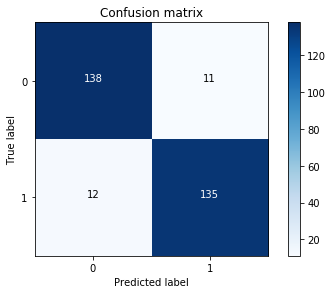
# 以下用向下采样处理后的数据集训练模型,并使用该数据集中分割出来的测试集进行测试

import itertools  #itertools 是python的迭代器模块,itertools提供的工具相当高效且节省内存。

# 创建&训练Logistic Regression模型并预测
lr = LogisticRegression(C = best_c, penalty = 'l1',solver='liblinear')
lr.fit(X_train_undersample,y_train_undersample.values.ravel())
y_pred_undersample = lr.predict(X_test_undersample.values)

# Compute confusion matrix
# 计算混淆矩阵
cnf_matrix = confusion_matrix(y_test_undersample,y_pred_undersample)
print("混淆矩阵:\n",cnf_matrix,"\n",type(cnf_matrix),"\n")
np.set_printoptions(precision=2)   #输出的精度,即小数点后位数,默认8

print("Recall metric in the testing dataset: ", cnf_matrix[1,1]/(cnf_matrix[1,0]+cnf_matrix[1,1]))

# Plot non-normalized confusion matrix
class_names = [0,1]
plt.figure()
plot_confusion_matrix(cnf_matrix
                      , classes=class_names
                      , title='Confusion matrix')
plt.show()
混淆矩阵:
 [[138  11]
 [ 12 135]]
 <class 'numpy.ndarray'>

Recall metric in the testing dataset:  0.9183673469387755
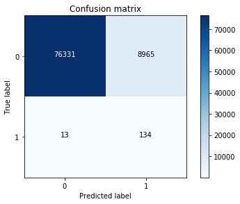
# 以下用向下采样处理后的数据集训练模型,并使用原始数据中分割出来的测试集进行测试

lr = LogisticRegression(C = best_c, penalty = 'l1',solver='liblinear')
lr.fit(X_train_undersample,y_train_undersample.values.ravel())
y_pred = lr.predict(X_test.values)

# Compute confusion matrix
cnf_matrix = confusion_matrix(y_test,y_pred)
np.set_printoptions(precision=2)

print("Recall metric in the testing dataset: ", cnf_matrix[1,1]/(cnf_matrix[1,0]+cnf_matrix[1,1]))

# Plot non-normalized confusion matrix
class_names = [0,1]
plt.figure()
plot_confusion_matrix(cnf_matrix
                      , classes=class_names
                      , title='Confusion matrix')
plt.show()
Recall metric in the testing dataset: 0.9115646258503401
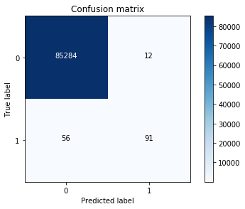
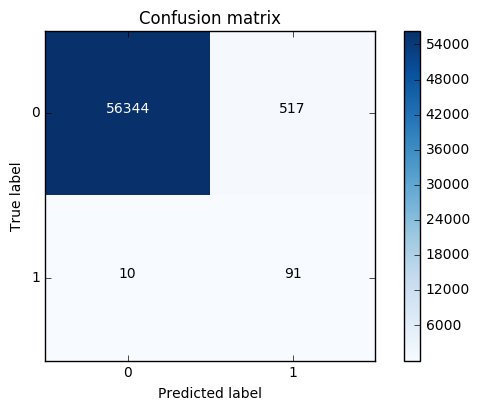
#下面不对原始数据作向下采样处理,并直接训练模型。分析模型和混淆矩阵
best_c = printing_Kfold_scores(X_train,y_train)
-------------------------------------------
C parameter:  0.01
-------------------------------------------

Iteration  1 : recall score =  0.4925373134328358
Iteration  2 : recall score =  0.6027397260273972
Iteration  3 : recall score =  0.6833333333333333
Iteration  4 : recall score =  0.5692307692307692
Iteration  5 : recall score =  0.45

Mean recall score  0.5595682284048672

-------------------------------------------
C parameter:  0.1
-------------------------------------------

Iteration  1 : recall score =  0.5671641791044776
Iteration  2 : recall score =  0.6164383561643836
Iteration  3 : recall score =  0.6833333333333333
Iteration  4 : recall score =  0.5846153846153846
Iteration  5 : recall score =  0.525

Mean recall score  0.5953102506435158

-------------------------------------------
C parameter:  1
-------------------------------------------

Iteration  1 : recall score =  0.5522388059701493
Iteration  2 : recall score =  0.6164383561643836
Iteration  3 : recall score =  0.7166666666666667
Iteration  4 : recall score =  0.6153846153846154
Iteration  5 : recall score =  0.5625

Mean recall score  0.612645688837163

-------------------------------------------
C parameter:  10
-------------------------------------------

Iteration  1 : recall score =  0.5522388059701493
Iteration  2 : recall score =  0.6164383561643836
Iteration  3 : recall score =  0.7333333333333333
Iteration  4 : recall score =  0.6153846153846154
Iteration  5 : recall score =  0.575

Mean recall score  0.6184790221704963

-------------------------------------------
C parameter:  100
-------------------------------------------

Iteration  1 : recall score =  0.5522388059701493
Iteration  2 : recall score =  0.6164383561643836
Iteration  3 : recall score =  0.7333333333333333
Iteration  4 : recall score =  0.6153846153846154
Iteration  5 : recall score =  0.575

Mean recall score  0.6184790221704963

   C_parameter Mean recall score
0         0.01          0.559568
1         0.10           0.59531
2         1.00          0.612646
3        10.00          0.618479
4       100.00          0.618479

*********************************************************************************
Best model to choose from cross validation is with C parameter =  10.0
*********************************************************************************
lr = LogisticRegression(C = best_c, penalty = 'l1',solver='liblinear')
lr.fit(X_train,y_train.values.ravel())
y_pred_undersample = lr.predict(X_test.values)

# Compute confusion matrix
cnf_matrix = confusion_matrix(y_test,y_pred_undersample)
np.set_printoptions(precision=2)

print("Recall metric in the testing dataset: ", cnf_matrix[1,1]/(cnf_matrix[1,0]+cnf_matrix[1,1]))

# Plot non-normalized confusion matrix
class_names = [0,1]
plt.figure()
plot_confusion_matrix(cnf_matrix
                      , classes=class_names
                      , title='Confusion matrix')
plt.show()

# 可以看到,用未处理的数据进行直接训练得到的模型,召回率偏低、误杀率偏高
Recall metric in the testing dataset: 0.6190476190476191
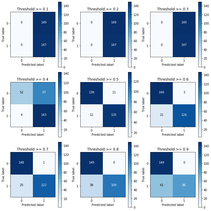
# 下面尝试用向下采样处理后的数据集进行训练、并对比不同阈值对分类效果的影响

lr = LogisticRegression(C = 0.01, penalty = 'l1',solver='liblinear')
lr.fit(X_train_undersample,y_train_undersample.values.ravel())
y_pred_undersample_proba = lr.predict_proba(X_test_undersample.values)
print("每一个样本对应的预测值:\n",y_pred_undersample_proba[0:5,:])

# 定义一个阈值
thresholds = [0.1,0.2,0.3,0.4,0.5,0.6,0.7,0.8,0.9]

plt.figure(figsize=(10,10))

j = 1
for i in thresholds:
    y_test_predictions_high_recall = y_pred_undersample_proba[:,1] > i

    plt.subplot(3,3,j)
    j += 1

    # Compute confusion matrix
    cnf_matrix = confusion_matrix(y_test_undersample,y_test_predictions_high_recall)
    np.set_printoptions(precision=2)

    print("Recall metric in the testing dataset: ", cnf_matrix[1,1]/(cnf_matrix[1,0]+cnf_matrix[1,1]))

    # Plot non-normalized confusion matrix
    class_names = [0,1]
    plot_confusion_matrix(cnf_matrix
                          , classes=class_names
                          , title='Threshold >= %s'%i)
每一个样本对应的预测值:
 [[0.57 0.43]
 [0.57 0.43]
 [0.   1.  ]
 [0.59 0.41]
 [0.54 0.46]]
Recall metric in the testing dataset:  1.0
Recall metric in the testing dataset:  1.0
Recall metric in the testing dataset:  1.0
Recall metric in the testing dataset:  0.9727891156462585
Recall metric in the testing dataset:  0.9183673469387755
Recall metric in the testing dataset:  0.8571428571428571
Recall metric in the testing dataset:  0.8299319727891157
Recall metric in the testing dataset:  0.7414965986394558
Recall metric in the testing dataset:  0.5850340136054422
#####################################向上采样策略:SMOTE方法 训练模型效果比较############################################
import pandas as pd

from imblearn.over_sampling import SMOTE   #SMOTE数据生成算法、即向上采样策略
from sklearn.ensemble import RandomForestClassifier
from sklearn.metrics import confusion_matrix
from sklearn.model_selection import train_test_split
credit_cards=pd.read_csv('creditcard.csv')

columns=credit_cards.columns
# The labels are in the last column ('Class'). Simply remove it to obtain features columns
# 删除最后一列,最后一列索引( len(columns)-1 )
features_columns=columns.delete(len(columns)-1)

# 从原始数据分离出特征 和 标签
features=credit_cards[features_columns]
labels=credit_cards['Class']
# 将数据分成训练集 和 测试集
features_train, features_test, labels_train, labels_test = train_test_split(features,
                                                                            labels,
                                                                            test_size=0.2,
                                                                            random_state=0)
len(labels_train)
227845
oversampler=SMOTE(random_state=0)
# 将训练数据传入,算法将会根据label值自动平衡并生成新的数据
os_features,os_labels=oversampler.fit_sample(features_train,labels_train)
len(os_labels[os_labels==1])
227454
os_features = pd.DataFrame(os_features)
os_labels = pd.DataFrame(os_labels)
best_c = printing_Kfold_scores(os_features,os_labels)
-------------------------------------------
C parameter:  0.01
-------------------------------------------

Iteration  1 : recall score =  0.8903225806451613
Iteration  2 : recall score =  0.8947368421052632
Iteration  3 : recall score =  0.9688170853159235
Iteration  4 : recall score =  0.9578263593497544
Iteration  5 : recall score =  0.9584198898671151

Mean recall score  0.9340245514566435

-------------------------------------------
C parameter:  0.1
-------------------------------------------

Iteration  1 : recall score =  0.8903225806451613
Iteration  2 : recall score =  0.8947368421052632
Iteration  3 : recall score =  0.9704105344694036
Iteration  4 : recall score =  0.9599366900781482
Iteration  5 : recall score =  0.9605631945131401

Mean recall score  0.9351939683622232

-------------------------------------------
C parameter:  1
-------------------------------------------

Iteration  1 : recall score =  0.8903225806451613
Iteration  2 : recall score =  0.8947368421052632
Iteration  3 : recall score =  0.9705211906606175
Iteration  4 : recall score =  0.9596069509018367
Iteration  5 : recall score =  0.9607830206306811

Mean recall score  0.9351941169887119

-------------------------------------------
C parameter:  10
-------------------------------------------

Iteration  1 : recall score =  0.8903225806451613
Iteration  2 : recall score =  0.8947368421052632
Iteration  3 : recall score =  0.9705211906606175
Iteration  4 : recall score =  0.9601894901133203
Iteration  5 : recall score =  0.9601455248898122

Mean recall score  0.9351831256828349

-------------------------------------------
C parameter:  100
-------------------------------------------

Iteration  1 : recall score =  0.8903225806451613
Iteration  2 : recall score =  0.8947368421052632
Iteration  3 : recall score =  0.970366271992918
Iteration  4 : recall score =  0.9594091073960497
Iteration  5 : recall score =  0.960530220595509

Mean recall score  0.9350730045469803

   C_parameter Mean recall score
0         0.01          0.934025
1         0.10          0.935194
2         1.00          0.935194
3        10.00          0.935183
4       100.00          0.935073

*********************************************************************************
Best model to choose from cross validation is with C parameter =  1.0
*********************************************************************************
lr = LogisticRegression(C = best_c, penalty = 'l1')
lr.fit(os_features,os_labels.values.ravel())
y_pred = lr.predict(features_test.values)

# Compute confusion matrix
cnf_matrix = confusion_matrix(labels_test,y_pred)
np.set_printoptions(precision=2)

print("Recall metric in the testing dataset: ", cnf_matrix[1,1]/(cnf_matrix[1,0]+cnf_matrix[1,1]))

# Plot non-normalized confusion matrix
class_names = [0,1]
plt.figure()
plot_confusion_matrix(cnf_matrix
                      , classes=class_names
                      , title='Confusion matrix')
plt.show()
Recall metric in the testing dataset: 0.90099009901
#Summary
# 对于样本不均匀的情况:
#  1、 利用下采样策略
#  2、利用SMOTE数据生成算法
#建议:数据利用越多越好。优先使用SMOTE数据生成算法


 815
815


 被折叠的 条评论
为什么被折叠?
被折叠的 条评论
为什么被折叠?
 到【灌水乐园】发言


