MATLAB基本绘图

最新推荐文章于 2022-09-02 01:33:23 发布

龟乐：分享有价

最新推荐文章于 2022-09-02 01:33:23 发布

阅读量1.2k

点赞数 2

分类专栏： matlab基础代码文章标签： matlab

本文链接：https://blog.csdn.net/qq_41878195/article/details/116168050

版权

matlab基础代码专栏收录该内容

2 篇文章

订阅专栏

本文展示了如何在MATLAB中绘制常数变量图像并生成图例，包括一维纯对流方程的解析解与迎风法求解的图像。通过示例代码，解释了如何控制曲线形状、去除图例边框以及自定义颜色和标记。此外，还讨论了图例在不同场景下的应用问题及其解决方案。

摘要生成于 C知道，由 DeepSeek-R1 满血版支持，前往体验 >

常数变量图像绘制及图例生成

MATLAB简单代码

% This is a demo
%例子：y=kx（k=1,2,3等任意常数）同时绘制在一张图中且生成每条线的图例
x = -10:10;
k = [1 2 3];
color = ['k' 'b' 'r'];
tuli=['y=kx'; 'y=2x';'y=3x'];%分号起到换行作用
for i=1:3
y = k(i).*x;
plot(x,y,color(i),'LineWidth',1.2); %color数组是为了自己指定每条线的颜色，否则三条线的颜色由系统默认
hold on %该语句很重要，否则无法生成三条直线
end
% % legend('y=kx','y=2x','y=3x','Location','NorthWest'); %按照函数图像绘制的先后顺序依次命名
legend(tuli,'Location','NorthWest'); %与上一语句效果相同
xlabel('x');
ylabel('y');

示例图像

在这里插入图片描述

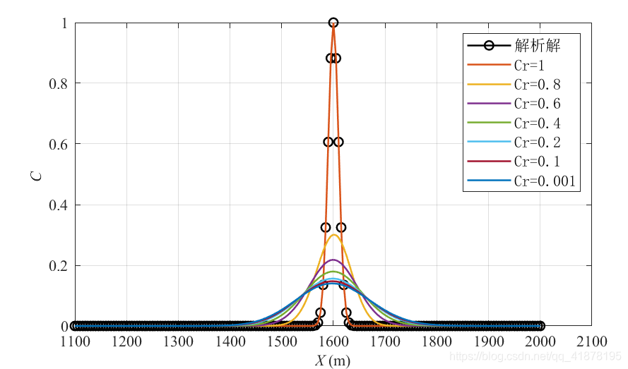
一维纯对流方程中遇到的图例显示问题

上述图例的使用方法在该实例中出错。

% This is a  First Order Upwind for Advection Equation 
clear
clc

% Set the parameters
xmin = 0;
xmax = 2000;
N = 400;
dx = (xmax-xmin)/N;
tmin = 0;
tmax = 1000;
dt = [5 4 3 2 1 0.5  0.005];
u = 1;
sigma = 10;
x0 = 600;
nstep = tmax./dt;

% Set the initial condition
x = linspace(xmin, xmax, N+1);
C0 = exp( -(x-x0).^2/sigma^2*0.5);
C0(1) = 0; %MATLAB Array index start from 1

Cexact = exp( -(x-x0-u*tmax).^2/sigma^2*0.5);%实际上此处的x应该足够小以完整刻画出真实曲线，而不是用离散时采用的空间步长
plot(x,Cexact,'k-o','linewidth',1.2);
hold on

for j = 1:7
    Cyf = C0;%给迎风法的变量赋初值
    for n = 1:nstep(j)
        Ctemp = Cyf;
        for i = 2:N+1
            Cyf(i) = Ctemp(i) - u*dt(j)*(Ctemp(i) - Ctemp(i-1))/dx;
        end
    end
    plot(x,Cyf,'-','linewidth',1.2);
    hold on
end

legend('解析解','Cr=1','Cr=0.8','Cr=0.6','Cr=0.4','Cr=0.2','Cr=0.1','Cr=0.001','location','NorthEast','FontName','宋体','Fontsize',10.5);

%tuli =['Cr=1';'Cr=1';'Cr=0.8';'Cr=0.6';'Cr=0.4';'Cr=0.2'];
%用这种表示方法会报错，说数组维度不一致

xlabel('\itX \rm(m)');
ylabel('\itC \rm');
axis([1100 2100 0 1]);
set(gca,'FontName','Times New Roman','Fontsize',10.5);
set(get(gca,'xlabel'),'FontName','Times New Roman','Fontsize',10.5);
set(get(gca,'ylabel'),'FontName','Times New Roman','Fontsize',10.5);
grid on;
set(gcf,'PaperUnits','centimeter','PaperPosition',[0 0 16 9]);
% print(figure(1),'-dtiff','-r300','fig_7_1');
%saveas(gcf,'具体的保存地址\sigma0=10.tif');

在这里插入图片描述

绘图曲线形状控制与图例边框去除

绘图曲线形状控制
在这里插入图片描述

load census;
x = [1.0 0.8 0.6 0.4 0.2 0.1 0.001];
y1 =1 - [1.0000 0.3011 0.2182 0.1795 0.1561 0.1474 0.1400];
y2 =1 - [1.0000 0.8669 0.7759 0.7085 0.6562 0.6340 0.6141];
y3 =1 - [1.0000 0.9535 0.9129 0.8770 0.8451 0.8305 0.8167];

plot(x,y1,'r-.o','MarkerFaceColor','r','LineWidth',1.2)
hold on
plot(x,y2,'k-.pentagram','MarkerFaceColor','k','LineWidth',1.2)
hold on
plot(x,y3,'b-.square','MarkerFaceColor','b','LineWidth',1.2)

xlabel('\itCr \rm');
ylabel('\itCe \rm');
legend('\sigma0=10','\sigma0=55','\sigma0=100','location','NorthEast','FontName','宋体');
set(tuli,'Box','off');

set(gca,'FontName','Times New Roman','Fontsize',10.5);
set(get(gca,'xlabel'),'FontName','Times New Roman','Fontsize',10.5);
set(get(gca,'ylabel'),'FontName','Times New Roman','Fontsize',10.5);
title('不同边界条件下计算峰值误差曲线','FontName','宋体','Fontsize',12);
grid on;
set(gcf,'PaperUnits','centimeter','PaperPosition',[0 0 16 9]);
saveas(gcf,'具体保存位置\不同边界条件下峰值误差曲线.tif');