FIR versus IIR & Butterworth & Chebyshev & Bessel Filter

最近在看FBCSP的代码，发现用到了滤波器，然后就学习了一下，就……一发不可收拾，内容有点多，scipy这个库里的函数太多了，直接给看蒙了。一劳永逸吧，整理好方便以后查阅。

Introduction to Filters: FIR versus IIR

1. 引言

滤波器在数据采集和分析中具有很多应用，它们通过减小或放大某些频率来改变时间信号的频率成分。

例如，如Figure 1所示，低通滤波器以三种不同的方式影响信号中的频率成分：一些频率成分保持不变，而其它频率成分的幅度变小或从信号中完全移除.。

Figure 1: A low pass filter passes low frequencies unaltered (left) and removes high frequencies (right)  

滤波器还可以放大特定的频带，而不仅仅是减弱或删除部分频带. 滤波器调整信号的幅度可以用线性形式表示(即放大系数）或增益/衰减分贝，如Figure 2所示。

Figure 2: Left graph – Linear filter amplitude in multiplication factor versus frequency, Right graph – Same filter in decibel scale of attenuation versus frequency  

线性度量指标和分贝度量指标有以下等价关系：

1. 线性振幅的1/2代表6分贝的衰减
2. 没有调整的频带对应线性增益为1，或0分贝衰减

虽然在频域查看滤波器特性很有用，但是滤波器是在时域进行工作的(Figure 3)。

Figure 3: An input signal with high frequency noise is passed through a low pass filter. The resulting output has the high frequency noise removed, resulting in a clean signal  

滤波器以时域信号为输入，修改频率内容，得到新的时域信号.

2. 滤波器的应用(Applications of Filters)

滤波器可用于信号清理与信号分析. 在某些应用中，滤波器用于通过衰减不需要的频率内容来调节时域信号. 例如：

• 抗混叠滤波器(Anti-Aliasing Filter)—抗混叠滤波器用于去除模拟数字转换前不能正确数字化的信号频带
• 去噪(Noise Removal)—可以用来去除信号中不需要的高频噪声，例如在音乐录音中的呲呲声
• 漂移消除(Drift Removal)—通过高通滤波器或交流耦合器(AC coupling)从信号中消除漂移或较大的偏移

有时滤波器用于将特定的信号特性保留下来用于后续分析:

• A加权(A-Weighting)—A加权滤波器(Figure 4)用于将人的听觉特性引入麦克风数据采集. 麦克风在听不同频率的信号时，其状态是一样的，即无法区分不同的频率输入，而人耳却能感觉到不同频率信号的差异. A加权滤波器降低麦克风采集信号的高频和低频部分，以模拟人耳感知声音的方式

Figure 4: A-weighting filter frequency domain shape. Y-axis is gain or attenuation in dB versus X-axis in frequency  

• 全身振动加权(Whole Body Vibration Weighting)—人体对某些特定的振动频率比较敏感，因此，基于加速度计的振动信号，结合全身振动加权滤波器(ISO 2631)可以对人体的健康和舒适度进行评价

滤波器可应用于模拟系统(针对实时信号)，或数字系统(针对PC上已记录的信号).

3. 滤波器类型(Filter Types)

滤波器可以针对不同的任务进行设计. 例如，滤波器可以分为高通(high pass)、低通(low pass)、带阻(band stop)或带通(band pass)滤波器(Figure 5).

Figure 5: Types of Filters  

滤波器类型:

• 高通滤波器—高通滤波器用于去除信号中的低频偏移. 例如，如果仅对应变仪信号的动态内容感兴趣，则可以使用高通滤波器去除仪表中的任何低频漂移
• 低通滤波器—低通滤波器衰减或消除指定频率以上的频率. 例如，其可以用来去除音频记录中的高频嘶嘶声
• 带通滤波器—此滤波器用于仅允许指定频率范围内的信号通过滤波器
• 带阻滤波器—带阻滤波器用于去除指定范围内的信号频率

这些滤波器类型可以使用FIR或IIR滤波器来实现, 也可以使用这些组合来生成任意形状的滤波器.

4. FIR和IIR(FIR versus IIR)

两类数字滤波器是有限脉冲响应(Finite Impulse Response, FIR)和无限脉冲响应(Infinite Impulse Response , IIR).

脉冲响应(Impulse Response) 是指滤波器在时域内的表现，滤波器通常具有较宽的频率响应，这对应于时域内的短时间脉冲，如Figure 6所示.

Figure 6: Frequency (left) and time (right) domain representations of filter shape  

IIR和FIR滤波器的方程如Equation 1所示. 滤波器的输入为时间序列$x(n)$，滤波器的输出为时间序列$y(n)$. 第一个样本点在$n=0$处。

Equation 1: Finite Impulse Response (FIR) filter equations versus Infinite Impulse Response (IIR) filter  

IIR和FIR实现之间的数学区别在于IIR滤波器使用一些滤波器的输出作为输入， 这使得IIR滤波器成为一个递归函数。

每个方程都有三个数字序列: 输入时间序列、滤波器和输出时间序列(Figure 7).

• $x(n)$—输入时间序列是$x(0),x(1),x(2),...,x(n)$. 小写$n$是输入时间序列中数据点的总数
• $a(k)$—FIR滤波器用字符“$a$” 表示，IIR滤波器用字符“$a$”和“$b$”. 大写字母$N$和$P$分别表示滤波器中的项数，也称为滤波器的阶数
• $y(n)$—输出时间序列$y(0),y(1),y(2),\dots$

Figure 7: Time series for input time history, “x(n)”, FIR filter - Series “a(k)”, and output time history, “y(n)”  

在实践中，FIR和IIR滤波器具有重要的性能差异，如Figure 8所示.

Figure 8: Summary of differences between IIR and FIR filters  

IIR滤波器的优点是，对于与FIR类似的滤波器，可以使用较低的阶数或项数. 这意味着实现相同结果所需的计算量更少，使得IIR的计算速度更快.

然而，IIR具有非线性相位和稳定性问题. 这有点像龟兔赛跑的寓言，FIR滤波器就像赛跑中的乌龟—缓慢而稳定，总是能跑完全程. 兔子就像IIR滤波器—非常快，但有时崩溃，并没有完成比赛.

4.1. 滤波器阶数和计算速度(Filter Order and Computational Speed)

由Equation 1中的FIR滤波器方程可知，N越大，滤波器的阶数越高. 例如，如果滤波器项数为10，而不是5，那么滤波器的计算将花费两倍的时间。然而，滤波器的频率下降会更清晰，如Figure 9所示.

Figure 9: Top – The roll off sharpness of the filter (top) with fewer terms is less sharp than filter with more terms (bottom)  

包含更多项(阶数更高)滤波器在通过频率和截止频率之间有更明显的转换.

Figure 10显示了相同滤波器类型在使用不同阶数计算时的幅频响应图.

Figure 10: Increasing the order of filter, but keeping all else the same, increases the sharpness of the filter roll off  

通过增加阶数来使滤波器转换段更陡峭。这需要更多的计算，并且对滤波器引入的时间延迟有影响。

阶数越高，滤波器的幅频响应变化曲线越陡峭，滤波器对滤除的频率截断效果越显著.

对于相同的阶数，FIR和IIR滤波器的锐度差别很大，如Figure 11所示. 由于IIR滤波器的递归性质(Equation 1)，其中部分滤波器输出用作输入，它可以使用相同阶的滤波器实现更陡峭的增益变化.

Figure 11: For the same order, the IIR filter has a sharper roll off than a FIR filter  

因此，IIR可以使用更少的阶数来实现与FIR相同的性能，如Figure 12所示.

Figure 12: An IIR filter can achieve similar performance to a FIR filter with a lower order  

从计算的角度来看，这使得IIR滤波器比FIR滤波器更快. 如果必须在实时应用程序中实现滤波器(例如在监听时进行交互过滤)，通常选择IIR.

然而，使用IIR滤波器也有一些潜在的缺点:

• 延迟—IIR在不同频率下的延迟不同，而FIR在每个频率的延迟一致
• 稳定性—由于其结构的特殊性，IIR滤波器有时可能是不稳定的，可能出现无法计算或应用于数据的情况，而FIR滤波器的计算始终是稳定的

即想要达到相同的滤波效果，IIR滤波器所需的阶数更少，计算量更小，速度也就更快.

4.2. 滤波器的时间延迟(Time Delay)

滤波后的时间序列，与原始时间序列相比，会出现轻微的偏移或时间延迟. Figure 13显示了同步采集的声音数据(红色曲线，顶部)和振动数据(蓝色曲线，底部). 对声音数据滤波器后(绿色曲线，顶部)会导致声音和振动数据之间出现时延现象.

Figure 13: Top - Original time signal (red) is time delayed (green) by filter. Bottom – Vibration signal (blue) no longer aligned with filtered sound signal (green)  

在某些应用程序中，这不是问题，因为偏移量是已知的，可以忽略.

而在其他应用中，这种延迟可能很重要. 例如:

• 故障排除(Troubleshooting)—对于多通道的声音和振动数据，如果只对声音通道使用滤波器，相对于振动通道，滤波后的声音会引入一个时间延迟(见图13底部图). 当试图确定一个振动事件是否产生了一个声音时，这一次的不对齐将很难看到振动和声音事件是否相关
• 运行变形振型(Operational Deflection Shapes)—如果运行变形振型中的某些振动通道使用了滤波器，而其它通道没有，这将导致这些通道之间的相位关系发生改变，结果其显示的波形将不正确

是什么原因导致滤波器在输出时间序列中引入了时间延迟?

从Figure 14中得到FIR滤波器的方程，通过对该方程的分析，可以看出产生时延的原因.

Figure 14: To be fully realized (i.e., actually work) the filter requires as many data points (n) as the terms (N) to be passed through the filter  

输入信号(x)中的一些时间序列样本必须通过与项数(N)成比例的滤波器，然后滤波器才会工作。此外，在输入滤波器的样本点数(n)大于N以前，滤波后的时间序列不会开始输出.

因为必须先有一些数据通过滤波器才能创建输出，所以与输入时间序列(x)相比，输出时间序列(y)的创建会有一个延迟，如Figure 13所示. 滤波器的幅频响应变化曲线越陡峭锐利，这种延迟就越长.

FIR和IIR滤波器的延迟特性有很大的不同，如图15所示.

Figure 15: IIR and FIR Filter amplitude (top) and time delay (bottom). A FIR has equal delay at all frequencies while the IIR filter time delay varies with frequency  

FIR滤波器在所有频率上具有相同的时延，而IIR滤波器的时延随频率而变化. 通常IIR滤波器中最大的时延出现在滤波器的截止频率处.

FIR滤波器在所有频率上具有相同的时延，而IIR滤波器的时延随频率而变化.

所有的滤波器都会产生某种时延(模拟或数字)，根据滤波器的特性，延迟或长或短，它们也可以是频率的函数.

4.3. 零相位滤波(Zero Phase)

通过“前向和后向”滤波，输出时间序列中的时延可以被消除. 在对x(n)滤波得到输出y(n)之后，可以对y(n)再次进行滤波，首先将y(n)中的数据点反转，再输入滤波器进行滤波. 这就是所谓的零相位滤波(zero phase filtering)，结果如Figure 16所示.

Figure 16: Original signal (red) filtered directly (green) and with zero phase (blue). Zero phase removes the delay, but data is lost at the end of zero phase filtered time history  

注意，时间延迟位于零相位滤波输出的末尾(蓝色).

零相位滤波的输出y(n)与x(n)实现了对齐，但数据由于滤波了两次，衰减加倍. 当使用零相位滤波器时，需要进行以下权衡:

• 计算时间加倍
• 针对数字信号的实现比较容易，针对模拟信号并不是
• 输出序列末尾的样本点被消除了

5. 滤波器属性(Filter Methods and Attributes)

可以选择滤波器的系数a(n)来控制特定的滤波器属性，如Figure 17所示.

Figure 17: Pass, Transition, and Stop band  

滤波器有四个主要的属性:

• 通频带(Pass Band)–通频带中的数据直接输出到输出时间序列. 为了保证通频带内的数据与原始时程数据一致，滤波器中不应有纹波. 纹波是振幅随频率的微小变化，理想情况下，在这个波段，滤波器的振幅应该恰好为1.
• 过渡带宽(Transition Width)–根据应用程序的不同，可能希望通过和截止频带之间的转换在频率方面尽可能窄，该方法和滤波器的阶数决定了通带和截止带之间转换发生的速度.
• 截止频带(Stop Band)–如果滤波器有纹波，截止带也可以包含输出数据. 在某些应用中，纹波的存在可能无关紧要，而在某些特定的场合下，则不能接受纹波的存在.
• 群时延(Group Delay/Phase)–滤波器在输出时间序列中引入了时延，该时延可能是随频率变化的函数. 如前所述，通过前向和后向滤波器(零相位滤波器)可以消除输出时间序列中的时延现象. 在某些应用程，相位也是很重要的，此时就不能再用零相位滤波器了.

5.1 FIR滤波方法(FIR Filter Methods)

下面列出了有限脉冲响应(FIR)滤波器的方法，如Figure 18所示.

Figure 18: FIR Filter Methods  

FIR方法在从频域到时域的转换中使用了不同的谱窗。一些窗口方法包括:

• Chebyshev - 停止带纹波最小，过渡带最宽
• Hamming - 过渡区窄，波纹比Hanning小
• Kaiser - 在停止区有较小的纹波
• Hanning - 过渡带最窄，停止带纹波较大
• Rectangular - 纹波最大，甚至影响通带

5.2 IIR滤波方法(IIR Filter Methods)

无限脉冲响应滤波器的方法如Figure 19所示.

Figure 19: Comparison of Low Pass IIR filters with same order and cutoff frequency  

不同IIR滤波方法的属性:

• Butterworth - 在通带和停止带响应平稳，但过渡区较宽
• Inverse Chebyshev - 通带平坦，过渡带宽度比巴特沃斯滤波器窄，但在停止带有波纹
• Chebyshev - 在通带可以有纹波，但其过渡带比反向Chebyshev更短
• Cauer - 过渡带最短，通带和停止带均有纹波
• Bessel - 在通带和停止带均出现幅度倾斜(Sloping)，过度带非常宽

A filter method can be selected to best suit a particular application.

Butterworth & Chebyshev & Bessel Filter

Butterworth

1.引言

这种滤波器最先由英国工程师斯蒂芬·巴特沃斯（Stephen Butterworth）在1930年发表在英国《无线电工程》期刊的一篇论文中提出的。

巴特沃斯（Butterworth）滤波器在现代设计方法设计的滤波器中，是最为有名的滤波器。

由于它设计简单，性能方面又没有明显的缺点，又因它对构成滤波器的元件Q值较低，因而易于制作且达到设计性能，因而得到了广泛应用。

其中，巴特沃斯滤波器的特点是通频带的频率响应曲线最平滑。

2.特点

巴特沃斯低通滤波器可用如下振幅的平方对频率的公式表示：

其中，$n$为滤波器的阶数，${\omega }_c$为截至频率，即振幅下降为$-3dB$时的频率，${\omega }_p$为通频带边缘频率。

下图为巴特沃斯滤波器的频率响应图

当$n->\infty$时，得到一个理想的低通滤波反馈: $\frac{\omega }{{\omega }_c}<1$ 时，增益为$1$；$\frac{\omega }{{\omega }_c}>1$ 时，增益为$0$；$\frac{\omega }{{\omega }_c}=1$ 时，增益为$0.707$

巴特沃斯滤波器的特点是通频带内的频率响应曲线最大限度平坦，没有起伏，而在阻频带则逐渐下降为零。

巴特沃斯滤波器的频率特性曲线，无论在通带内还是阻带内都是频率的单调函数。

因此，当通带的边界处满足指标要求时，通带内肯定会有裕量。所以，更有效的设计方法应该是将精确度均匀的分布在整个通带或阻带内，或者同时分布在两者之内。这样就可用较低阶数的系统满足要求。这可通过选择具有等波纹特性的逼近函数来达到。

3.Python代码

API reference —— butter

scipy.signal.butter(N, Wn, btype='low', analog=False, output='ba', fs=None)

'''
巴特沃斯数字和模拟滤波器设计。
设计一个 N 阶数字或模拟巴特沃斯滤波器并返回滤波器系数。
'''

输入参数：
N:滤波器的阶数

Wn：归一化截止频率。计算公式Wn=2*截止频率/采样频率。（注意：根据采样定理，采样频率要大于两倍的信号本身最大的频率，才能还原信号。临界频率或频率。对于低通和高通滤波器，Wn 是标量；对于带通和带阻滤波器，Wn 是长度为 2 的序列。
对于巴特沃斯滤波器，这是增益下降到通带增益的 1/sqrt(2) 的点（“-3 dB 点”）。
对于数字滤波器，如果未指定 fs，则 Wn 单位从 0 归一化为 1，其中 1 是奈奎斯特频率（Wn 因此以半周期/样本为单位，定义为 2*临界频率/fs）。如果指定了 fs，则 Wn 的单位与 fs 相同。
对于模拟滤波器，Wn 是角频率（例如 rad/s）。

analog: 如果为 True，则返回模拟滤波器，否则返回数字滤波器。默认返回数字滤波器。

btype: 滤波器类型{‘lowpass’, ‘highpass’, ‘bandpass’, ‘bandstop’},

output: 输出类型{‘ba’, ‘zpk’, ‘sos’}

fs: 数字系统的采样频率。

输出参数：
b，a: IIR滤波器的分子（b）和分母（a）多项式系数向量。output='ba'

z,p,k: IIR滤波器传递函数的零点、极点和系统增益. output= 'zpk'

sos: IIR滤波器的二阶截面表示。output= 'sos'

Example

Design an analog filter and plot its frequency response, showing the critical points:

import numpy as np
from scipy import signal
import matplotlib.pyplot as plt

b, a = signal.butter(4, 100, 'low', analog=True) # 模拟滤波器
w, h = signal.freqs(b, a) # 计算模拟滤波器的频率响应
plt.semilogx(w, 20 * np.log10(abs(h)))
plt.title('Butterworth filter frequency response')
plt.xlabel('Frequency [radians / second]')
plt.ylabel('Amplitude [dB]')
plt.margins(0, 0.1)
plt.grid(which='both', axis='both')
plt.axvline(100, color='green') # cutoff frequency
plt.show()

Generate a signal made up of 10 Hz and 20 Hz, sampled at 1 kHz

t = np.linspace(0, 1, 1000, False)  # 1 second
sig = np.sin(2*np.pi*10*t) + np.sin(2*np.pi*20*t)
fig, (ax1, ax2) = plt.subplots(2, 1, sharex=True)
ax1.plot(t, sig)
ax1.set_title('10 Hz and 20 Hz sinusoids')
ax1.axis([0, 1, -2, 2])

Design a digital high-pass filter at 15 Hz to remove the 10 Hz tone, and apply it to the signal. (It’s recommended to use second-order sections format when filtering, to avoid numerical error with transfer function (ba) format):

sos = signal.butter(10, 15, 'hp', fs=1000, output='sos') # 默认为数字滤波器

fig, ax = plt.subplots()
w, h = signal.sosfreqz(sos) # 以 SOS 格式计算数字滤波器的频率响应
plt.semilogx(w, 20 * np.log10(abs(h)))
plt.title('Butterworth filter frequency response')
plt.xlabel('Frequency [radians / second]')
plt.ylabel('Amplitude [dB]')
plt.margins(0, 0.1)
plt.grid(which='both', axis='both')
plt.axvline(100, color='green') # cutoff frequency

filtered = signal.sosfilt(sos, sig)
ax2.plot(t, filtered)
ax2.set_title('After 15 Hz high-pass filter')
ax2.axis([0, 1, -2, 2])
ax2.set_xlabel('Time [seconds]')
plt.tight_layout()
plt.show()

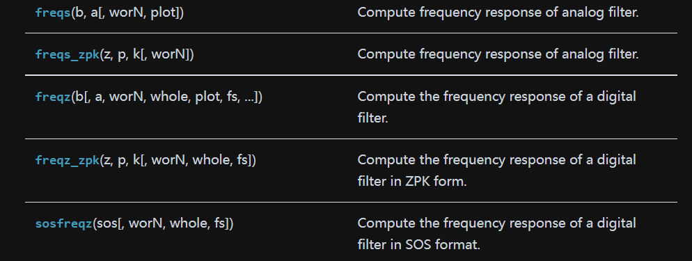
API reference —— freqs & freqz

API reference —— sosfilt

scipy.signal.sosfilt(sos, x, axis=- 1, zi=None)

'''
使用级联二阶部分沿一维过滤数据。
使用由 sos 定义的数字 IIR 滤波器对数据序列 x 进行滤波。
'''

输入参数：
sos： 二阶滤波器系数数组，必须具有形状 (n_sections, 6)。每行对应一个二阶部分，前三列提供分子系数，后三列提供分母系数。

x： 一个 N 维输入数组。

axis： 沿其应用线性滤波器的输入数据数组的轴。过滤器沿该轴应用于每个子阵列。默认值为 -1。

zi： 级联滤波器延迟的初始条件。它是一个形状为 (n_sections, ..., 2, ...) 的（至少 2D）向量，其中 ..., 2, ... 表示 x 的形状，但用 x.shape[axis] 替换乘以 2。如果 zi 为 None 或未给出，则假定初始休息（即全零）。请注意，这些初始条件与 lfiltic 或 lfilter_zi 给出的初始条件不同。

输出参数：
y： 数字滤波器的输出。

zf： 如果 zi 为 None，则不返回，否则，zf 保存最终的滤波器延迟值。

Example

Plot a 13th-order filter’s impulse response using both lfilter and sosfilt, showing the instability that results from trying to do a 13th-order filter in a single stage (the numerical error pushes some poles outside of the unit circle):

import matplotlib.pyplot as plt
from scipy import signal
b, a = signal.ellip(13, 0.009, 80, 0.05, output='ba')
sos = signal.ellip(13, 0.009, 80, 0.05, output='sos')
x = signal.unit_impulse(700)
y_tf = signal.lfilter(b, a, x)
y_sos = signal.sosfilt(sos, x)
plt.plot(y_tf, 'r', label='TF')
plt.plot(y_sos, 'k', label='SOS')
plt.legend(loc='best')
plt.show()

API reference —— lfilter

scipy.signal.lfilter(b, a, x, axis=- 1, zi=None)

'''
使用 IIR 或 FIR 滤波器沿一维过滤数据。
对于大多数过滤任务，函数 sosfilt（以及使用 output='sos' 的过滤器设计）应该优先于 lfilter，因为二阶部分的数值问题较少。
'''

输入参数：
b： 一维序列中的分子系数向量。

a： 一维序列中的分母系数向量。如果 a[0] 不是 1，则 a 和 b 都被 a[0] 归一化。

x： An N-dimensional input array.

axis： The axis of the input data array along which to apply the linear filter. The filter is applied to each subarray along this axis. Default is -1.

zi： Initial conditions for the filter delays. It is a vector (or array of vectors for an N-dimensional input) of length max(len(a), len(b)) - 1. If zi is None or is not given then initial rest is assumed. See lfiltic for more information.

输出参数：
y： The output of the digital filter.

zf： If zi is None, this is not returned, otherwise, zf holds the final filter delay values.

Example

Generate a noisy signal to be filtered:

from scipy import signal
import matplotlib.pyplot as plt
rng = np.random.default_rng()
t = np.linspace(-1, 1, 201)
x = (np.sin(2*np.pi*0.75*t*(1-t) + 2.1) +
     0.1*np.sin(2*np.pi*1.25*t + 1) +
     0.18*np.cos(2*np.pi*3.85*t))
xn = x + rng.standard_normal(len(t)) * 0.08

Create an order 3 lowpass butterworth filter:

b, a = signal.butter(3, 0.05)

Apply the filter to xn. Use lfilter_zi to choose the initial condition of the filter:

zi = signal.lfilter_zi(b, a)
z, _ = signal.lfilter(b, a, xn, zi=zi*xn[0])

Apply the filter again, to have a result filtered at an order the same as filtfilt:

z2, _ = signal.lfilter(b, a, z, zi=zi*z[0])

Use filtfilt to apply the filter:

y = signal.filtfilt(b, a, xn)

Plot the original signal and the various filtered versions:

plt.figure
plt.plot(t, xn, 'b', alpha=0.75)
plt.plot(t, z, 'r--', t, z2, 'r', t, y, 'k')
plt.legend(('noisy signal', 'lfilter, once', 'lfilter, twice',
            'filtfilt'), loc='best')
plt.grid(True)
plt.show()

API reference —— lfilter_zi

scipy.signal.lfilter_zi(b, a)

'''
为阶跃响应稳态构建 lfilter 的初始条件。
计算对应于阶跃响应稳态的 lfilter 函数的初始状态 zi。
此函数的典型用途是设置初始状态，以便滤波器的输出从与要滤波的信号的第一个元素相同的值开始。
'''

输入参数：
b, a： The IIR filter coefficients. See lfilter for more information.

输出参数：
zi： The initial state for the filter.

Example

The following code creates a lowpass Butterworth filter. Then it applies that filter to an array whose values are all 1.0; the output is also all 1.0, as expected for a lowpass filter. If the zi argument of lfilter had not been given, the output would have shown the transient signal.

from numpy import array, ones
from scipy.signal import lfilter, lfilter_zi, butter
b, a = butter(5, 0.25)
zi = lfilter_zi(b, a)
y, zo = lfilter(b, a, ones(10), zi=zi)

Another example:

x = np.array([0.5, 0.5, 0.5, 0.5, 0.5, 0.0, 0.0])
y, zf = signal.lfilter(b, a, x, zi=zi*x[0])
print(y)
y, zf = signal.lfilter(b, a, x, zi=zi)
print(y)

API reference —— filtfilt

scipy.signal.filtfilt(b, a, x, axis=-1, padtype='odd', padlen=None, method='pad', irlen=None)


'''
向前和向后对信号应用数字滤波器。
此功能应用线性数字滤波器两次，一次向前，一次向后。组合滤波器的相位为零，滤波器阶数是原始滤波器的两倍。
对于大多数过滤任务，函数 sosfiltfilt（以及使用 output='sos' 的过滤器设计）应该优于 filtfilt，因为二阶部分的数值问题较少。
'''

输入参数：
b: 滤波器的分子系数向量

a: 滤波器的分母系数向量

x: 要过滤的数据数组。（array型）

axis: 指定要过滤的数据数组x的轴

padtype: 必须是“奇数”、“偶数”、“常数”或“无”。这决定了用于应用滤波器的填充信号的扩展类型。如果 padtype 为 None，则不使用填充。默认值为“奇数”。

padlen：在应用过滤器之前在轴的两端扩展 x 的元素数。该值必须小于 x.shape[axis] - 1。padlen=0 表示没有填充。默认值为 3 * max(len(a), len(b))。

method：确定处理信号边缘的方法，“pad”或“gust”。当method为“pad”时，信号被填充； padding 的类型由 padtype 和 padlen 决定，irlen 被忽略。当 method 为“gust”时，使用 Gustafsson 的方法，忽略 padtype 和 padlen。

irlen：当 method 为“gust”时，irlen 指定滤波器的脉冲响应的长度。如果 irlen 为 None，则不会忽略任何部分的脉冲响应。对于长信号，指定 irlen 可以显着提高滤波器的性能。

输出参数：
y:滤波后的数据数组

Examples

The examples will use several functions from scipy.signal.

from scipy import signal
import matplotlib.pyplot as plt

First we create a one second signal that is the sum of two pure sine waves, with frequencies 5 Hz and 250 Hz, sampled at 2000 Hz.

fig, (ax1, ax2) = plt.subplots(2, 1, sharex=True)

t = np.linspace(0, 1.0, 2001)
xlow = np.sin(2 * np.pi * 5 * t)
xhigh = np.sin(2 * np.pi * 250 * t)
x = xlow + xhigh
ax1.plot(t, x)
ax1.set_title('5 Hz and 250 Hz sinusoids')
ax1.axis([0, 1, -2, 2])

Now create a lowpass Butterworth filter with a cutoff of 0.125 times the Nyquist frequency, or 125 Hz, and apply it to x with filtfilt. The result should be approximately xlow, with no phase shift.

b, a = signal.butter(8, 0.125)
y = signal.filtfilt(b, a, x, padlen=150)
ax2.plot(t, y)
ax2.set_title('After 125 Hz high-pass filter')
ax2.axis([0, 1, -2, 2])
ax2.set_xlabel('Time [seconds]')
plt.tight_layout()
plt.show()
print(np.abs(y - xlow).max())

对于这个人为的例子，我们得到了一个相当干净的结果，因为奇数扩展是精确的，并且在中等长度的填充下，滤波器的瞬态在达到实际数据时已经消散。通常，边缘处的瞬态效应是不可避免的。

The following example demonstrates the option method=“gust”.

First, create a filter.

b, a = signal.ellip(4, 0.01, 120, 0.125)  # Filter to be applied.

sig is a random input signal to be filtered.

rng = np.random.default_rng()
n = 60
sig = rng.standard_normal(n)**3 + 3*rng.standard_normal(n).cumsum()

Apply filtfilt to sig, once using the Gustafsson method, and once using padding, and plot the results for comparison.

fgust = signal.filtfilt(b, a, sig, method="gust")
fpad = signal.filtfilt(b, a, sig, padlen=50)
plt.plot(sig, 'k-', label='input')
plt.plot(fgust, 'b-', linewidth=4, label='gust')
plt.plot(fpad, 'c-', linewidth=1.5, label='pad')
plt.legend(loc='best')
plt.show()

The irlen argument can be used to improve the performance of Gustafsson’s method.

Estimate the impulse response length of the filter.

z, p, k = signal.tf2zpk(b, a)
eps = 1e-9
r = np.max(np.abs(p))
approx_impulse_len = int(np.ceil(np.log(eps) / np.log(r)))
print(approx_impulse_len)

Apply the filter to a longer signal, with and without the irlen argument. The difference between y1 and y2 is small. For long signals, using irlen gives a significant performance improvement.

x = rng.standard_normal(5000)
y1 = signal.filtfilt(b, a, x, method='gust')
y2 = signal.filtfilt(b, a, x, method='gust', irlen=approx_impulse_len)
print(np.max(np.abs(y1 - y2)))

API reference —— sosfiltfilt

scipy.signal.sosfiltfilt(sos, x, axis=- 1, padtype='odd', padlen=None)

'''
使用级联二阶部分的前向后向数字滤波器。
有关此方法的更多完整信息，请参阅 filtfilt。
'''

输入参数：
sos： 二阶滤波器系数数组，必须具有形状 (n_sections, 6)。每行对应一个二阶部分，前三列提供分子系数，后三列提供分母系数。

x： 要过滤的数据数组。

axis： 应用过滤器的 x 轴。默认值为 -1。

padtype： 必须是“奇数”、“偶数”、“常数”或“无”。这决定了用于应用滤波器的填充信号的扩展类型。如果 padtype 为 None，则不使用填充。默认值为“奇数”。

padlen： 在应用过滤器之前在轴的两端扩展 x 的元素数。该值必须小于 x.shape[axis] - 1。padlen=0 表示没有填充。默认值为：
3 * (2 * len(sos) + 1 - min((sos[:, 2] == 0).sum(),
                            (sos[:, 5] == 0).sum()))

输出参数：
y： 与 x 形状相同的过滤输出。

Examples

from scipy.signal import sosfiltfilt, butter
import matplotlib.pyplot as plt
rng = np.random.default_rng()

Create an interesting signal to filter.

n = 201
t = np.linspace(0, 1, n)
x = 1 + (t < 0.5) - 0.25*t**2 + 0.05*rng.standard_normal(n)

Create a lowpass Butterworth filter, and use it to filter x.

sos = butter(4, 0.125, output='sos')
y = sosfiltfilt(sos, x)

For comparison, apply an 8th order filter using sosfilt. The filter is initialized using the mean of the first four values of x.

from scipy.signal import sosfilt, sosfilt_zi
sos8 = butter(8, 0.125, output='sos')
zi = x[:4].mean() * sosfilt_zi(sos8)
y2, zo = sosfilt(sos8, x, zi=zi)

Plot the results. Note that the phase of y matches the input, while y2 has a significant phase delay.

plt.plot(t, x, alpha=0.5, label='x(t)')
plt.plot(t, y, label='y(t)')
plt.plot(t, y2, label='y2(t)')
plt.legend(framealpha=1, shadow=True)
plt.grid(alpha=0.25)
plt.xlabel('t')
plt.show()

4.MATLAB代码

API reference —— buttord

[N，Wn] = buttord(Wp, Ws, Rp, Rs, ‘s’)  

'''
求解滤波器的阶数N和3dB截止频率wc
'''

输入参数：
wp： 通带边界模拟频率（模拟角频率，单位是rad/s）

Ws： 阻带边界模拟频率（模拟角频率，单位是rad/s）

Rp： 通带纹波不超过Rp dB（单位是dB）
是描述通带波纹（起伏程度）的一个参量，通带纹波是指在滤波器的频响中通带的最大幅值和最小幅值之间的差值，正常的纹波一般小于1db。
通带波纹当然越小越好，这样通带内频率的幅度都基本稳定在单倍幅度上，因此Rp是允许的通带波纹的最大值。

Rs： 阻带衰减至少为Rs dB（单位是dB）
描述阻带衰减的一个参量
阻带衰减越大越好，衰减越大代表对不想要的信号频率成分的滤除效果越好，因此Rs是允许的需要达到的阻带衰减的最小值。

s’： 指的就是模拟滤波器，设计数字滤波器时就没有’s’这个参数了

API reference —— butter

[B,A] = butter(N, Wn, ‘ftype’, ‘s’) 

'''
求解N阶滤波器的具体参数B和A
'''

输入参数：
N： 滤波器阶数

Wn： 3dB截止模拟频率（单位rad/s，N和wc都是用buttord函数计算出来的）

ftype： - 滤波器类型‘’：
（1）当输入wc为一维向量时：
默认情况下设计的低通滤波器，设计高通滤波器的话令ftype=high
（2）当输入wc为二维向量[wcl,wcu]时：
默认情况下设计的带通滤波器，设计带阻滤波器的话令ftype=stop

API reference —— filter

y = filter(B,A,x)

'''
滤波函数
'''

x： 输入的有噪声的信号

B，A： 设计好的滤波器参数

Examples

采样频率为$1kHz$，频率为$3Hz$和$15Hz$的信号混叠，设计滤波器，去除信号的中的高频噪声。

代码如下：

t = 0:0.001:1; % 采样频率为1000

x1 = sin(2*pi*3*t); % 频率为3Hz的信号
x2 = sin(2*pi*15*t); % 频率为15Hz的信号

x = x1+x2;

Wp = 5/(1000/2);
Ws = 12/(1000/2);
Rp = 1;
Rs = 60;

[N, Wn] = buttord(Wp, Ws, Rp, Rs)
[B, A] = butter(N, Wn);
y = filter(B,A,x);

subplot(2,1,1)
plot(t, x)
subplot(2,1,2)
plot(t, y)

figure
[h,w] = freqz(B, A)
plot(w*10^3, 20*log10(abs(h)))
xlabel('Normalized Frequency (\times\pi rad/sample)')
ylabel('Magnitude (dB)')
axis([0, 100, -100, 20]);

Chebyshev

1.引言

切比雪夫滤波器，又名“车比雪夫滤波器”，是在通带或阻带上频率响应幅度等波纹波动的滤波器。

• 切比雪夫滤波器传递函数：

其中${\omega }_0$为期望截至频率,$n$为滤波器阶数。

• 切比雪夫不等式：

2.特点

1. 切比雪夫滤波器是在通带或阻带上频率响应幅度等波纹波动（通带平坦、阻带等波纹或是阻带平坦、通带等波纹）的滤波器，振幅特性在通带内是等波纹。

2. 切比雪夫滤波器在过渡带比巴特沃斯滤波器的衰减快，但频率响应的幅频特性不如后者平坦。

3. 切比雪夫滤波器和理想滤波器的频率响应曲线之间的误差最小，但是在通频带内存在幅度波动。

4. 在通带（或称“通频带”）上频率响应幅度等波纹波动的滤波器称为“I型切比雪夫滤波器”，在阻带（或称“阻频带”）上频率响应幅度等波纹波动的滤波器称为“II型切比雪夫滤波器”

3.Python代码

API reference —— iirfilter

scipy.signal.iirfilter(N, Wn, rp=None, rs=None, btype='band', analog=False, ftype='butter', output='ba', fs=None)

'''
IIR 数字和模拟滤波器设计给定阶数和临界点。
设计一个 N 阶数字或模拟滤波器并返回滤波器系数。
'''

输入参数：
N：int  过滤器的顺序。

Wn：array_like  标量或长度为2的序列给出了临界频率(由norm参数定义)。对于模拟滤波器，Wn是角频率(例如rad /s)。

rp：float, 可选参数
对于Chebyshev和椭圆滤波器，可在通带中提供最大纹波。(db)

rs：float, 可选参数
对于切比雪夫和椭圆滤波器，在阻带中提供最小的衰减。(db)

btype：{‘lowpass’, ‘highpass’, ‘bandpass’, ‘bandstop’}, 可选参数
过滤器的类型。默认值为‘lowpass’。

analog：bool, 可选参数
如果为True，则返回一个模拟滤波器，否则返回一个数字滤波器。

ftype：str, 可选参数
设计的IIR滤波器的类型：{Butterworth :‘butter’, Chebyshev I :‘cheby1’, Chebyshev II :‘cheby2’, Cauer/elliptic:‘ellip’, Bessel/Thomson:‘bessel’}

output：{‘ba’, ‘zpk’, ‘sos’}, 可选参数
输出类型：分子/分母(‘ba’)，pole-zero(‘zpk’)或second-order部分(‘sos’)。默认值为‘ba’。

fs：float  可选参数     数字系统的采样频率。
对于数字滤波器，Wn与fs的单位相同。默认情况下，fs为2 half-cycles /sample，因此将它们从0标准化为1，其中1是奈奎斯特频率。 (因此Wn在half-cycles /样本中。)

返回值：
b, a：ndarray，ndarray
IIR滤波器的分子(b)和分母(a)多项式。仅在以下情况下返回output='ba'。

z, p, k：ndarray，ndarray，float
IIR滤波器传递函数的零点，极点和系统增益。仅在以下情况下返回output='zpk'。

sos：ndarray
IIR滤波器的Second-order个部分表示。仅在以下情况下返回output=='sos'。

Examples

Generate a 17th-order Chebyshev II analog bandpass filter from 50 Hz to 200 Hz and plot the frequency response:

from scipy import signal
import matplotlib.pyplot as plt
b, a = signal.iirfilter(17, [2*np.pi*50, 2*np.pi*200], rs=60,
                        btype='band', analog=True, ftype='cheby2')
w, h = signal.freqs(b, a, 1000)
fig = plt.figure()
ax = fig.add_subplot(1, 1, 1)
ax.semilogx(w / (2*np.pi), 20 * np.log10(np.maximum(abs(h), 1e-5)))
ax.set_title('Chebyshev Type II bandpass frequency response')
ax.set_xlabel('Frequency [Hz]')
ax.set_ylabel('Amplitude [dB]')
ax.axis((10, 1000, -100, 10))
ax.grid(which='both', axis='both')
plt.show()

Create a digital filter with the same properties, in a system with sampling rate of 2000 Hz, and plot the frequency response. (Second-order sections implementation is required to ensure stability of a filter of this order):

sos = signal.iirfilter(17, [50, 200], rs=60, btype='band',
                       analog=False, ftype='cheby2', fs=2000,
                       output='sos')
w, h = signal.sosfreqz(sos, 2000, fs=2000)
fig = plt.figure()
ax = fig.add_subplot(1, 1, 1)
ax.semilogx(w, 20 * np.log10(np.maximum(abs(h), 1e-5)))
ax.set_title('Chebyshev Type II bandpass frequency response')
ax.set_xlabel('Frequency [Hz]')
ax.set_ylabel('Amplitude [dB]')
ax.axis((10, 1000, -100, 10))
ax.grid(which='both', axis='both')
plt.show()

API reference —— cheb2ord

scipy.signal.cheb2ord(wp, ws, gpass, gstop, analog=False, fs=None)

'''
Chebyshev II 型滤波器阶数选择。
返回最低阶数字或模拟切比雪夫 II 型滤波器的阶，该滤波器在通带中的损失不超过 gpass dB，并且在阻带中至少具有 gstop dB 衰减。
'''

输入参数：
wp, ws： 通带和阻带边缘频率。

gpass： 通带中的最大损耗 (dB)。

gstop： 阻带中的最小衰减 (dB)。

analog： 如果为 True，则返回模拟滤波器，否则返回数字滤波器。

fs： 数字系统的采样频率。

输出参数：
ord： 符合规格的切比雪夫 II 型过滤器的最低阶。

wn： Chebyshev 固有频率（“3dB 频率”）与 cheby2 一起使用以给出过滤结果。如果指定了 fs，则单位相同，并且 fs 也必须传递给 cheby2。

Examples

Design a digital bandstop filter which rejects -60 dB from 0.2*(fs/2) to 0.5*(fs/2), while staying within 3 dB below 0.1*(fs/2) or above 0.6*(fs/2). Plot its frequency response, showing the passband and stopband constraints in gray.

from scipy import signal
import matplotlib.pyplot as plt

N, Wn = signal.cheb2ord([0.1, 0.6], [0.2, 0.5], 3, 60)
b, a = signal.cheby2(N, 60, Wn, 'stop')
w, h = signal.freqz(b, a)
plt.semilogx(w / np.pi, 20 * np.log10(abs(h)))
plt.title('Chebyshev II bandstop filter fit to constraints')
plt.xlabel('Normalized frequency')
plt.ylabel('Amplitude [dB]')
plt.grid(which='both', axis='both')
plt.fill([.01, .1, .1, .01], [-3,  -3, -99, -99], '0.9', lw=0) # stop
plt.fill([.2,  .2, .5,  .5], [ 9, -60, -60,   9], '0.9', lw=0) # pass
plt.fill([.6,  .6,  2,   2], [-99, -3,  -3, -99], '0.9', lw=0) # stop
plt.axis([0.06, 1, -80, 3])
plt.show()

API reference —— cheby2

scipy.signal.cheby2(N, rs, Wn, btype='low', analog=False, output='ba', fs=None)

'''
Chebyshev II 型数字和模拟滤波器设计。
设计一个 N 阶数字或模拟 Chebyshev II 型滤波器并返回滤波器系数。
'''

输入参数：
N： 过滤器的顺序。

rs： 阻带所需的最小衰减。以分贝为单位指定，为正数。

Wn： 给出临界频率的标量或长度为 2 的序列。对于 II 型滤波器，这是过渡带中增益首先达到 -rs 的点。
对于数字滤波器，Wn 的单位与 fs 相同。默认情况下，fs 是 2 个半周期/样本，因此这些从 0 归一化到 1，其中 1 是奈奎斯特频率。 （因此，Wn 在半周期/样本中。）
对于模拟滤波器，Wn 是角频率（例如，rad/s）。

btype： {‘lowpass’, ‘highpass’, ‘bandpass’, ‘bandstop’}, optional，过滤器的类型。默认为“低通”。

analog： 如果为 True，则返回模拟滤波器，否则返回数字滤波器。

output： 输出类型：分子/分母（“ba”）、零极点（“zpk”）或二阶部分（“sos”）。默认为“ba”以实现向后兼容性，但“sos”应用于通用过滤。

fs： 数字系统的采样频率。

输出参数：
b, a： IIR 滤波器的分子 (b) 和分母 (a) 多项式。仅在 output='ba' 时返回。

z, p, k： IIR 滤波器传递函数的零点、极点和系统增益。仅在 output='zpk' 时返回。

sos： Second-order sections representation of the IIR filter. Only returned if output=='sos'.

Examples

Design an analog filter and plot its frequency response, showing the critical points:

from scipy import signal
import matplotlib.pyplot as plt

b, a = signal.cheby2(4, 40, 100, 'low', analog=True)
w, h = signal.freqs(b, a)
plt.semilogx(w, 20 * np.log10(abs(h)))
plt.title('Chebyshev Type II frequency response (rs=40)')
plt.xlabel('Frequency [radians / second]')
plt.ylabel('Amplitude [dB]')
plt.margins(0, 0.1)
plt.grid(which='both', axis='both')
plt.axvline(100, color='green') # cutoff frequency
plt.axhline(-40, color='green') # rs
plt.show()

Generate a signal made up of 10 Hz and 20 Hz, sampled at 1 kHz

t = np.linspace(0, 1, 1000, False)  # 1 second
sig = np.sin(2*np.pi*10*t) + np.sin(2*np.pi*20*t)
fig, (ax1, ax2) = plt.subplots(2, 1, sharex=True)
ax1.plot(t, sig)
ax1.set_title('10 Hz and 20 Hz sinusoids')
ax1.axis([0, 1, -2, 2])

Design a digital high-pass filter at 17 Hz to remove the 10 Hz tone, and apply it to the signal. (It’s recommended to use second-order sections format when filtering, to avoid numerical error with transfer function (ba) format):

sos = signal.cheby2(12, 20, 17, 'hp', fs=1000, output='sos')
filtered = signal.sosfilt(sos, sig)
ax2.plot(t, filtered)
ax2.set_title('After 17 Hz high-pass filter')
ax2.axis([0, 1, -2, 2])
ax2.set_xlabel('Time [seconds]')
plt.show()

4.MATLAB代码

%  Cheby1Filter.m
%  切比雪夫Ⅰ型滤波器的设计
%

clear;
close all;
clc;

fs = 1000; %Hz 采样频率
Ts = 1/fs;
N  = 1000; %序列长度
t = (0:N-1)*Ts;
delta_f = 1*fs/N;
f1 = 50;
f2 = 100;
f3 = 200;
f4 = 400;
x1 = 2*0.5*sin(2*pi*f1*t);
x2 = 2*0.5*sin(2*pi*f2*t);
x3 = 2*0.5*sin(2*pi*f3*t);
x4 = 2*0.5*sin(2*pi*f4*t);
x = x1 + x2 + x3 + x4; %待处理信号由四个分量组成

X = fftshift(abs(fft(x)))/N;
X_angle = fftshift(angle(fft(x)));
f = (-N/2:N/2-1)*delta_f;

figure(1);
subplot(3,1,1);
plot(t,x);
title('原信号');
subplot(3,1,2);
plot(f,X);
grid on;
title('原信号频谱幅度特性');
subplot(3,1,3);
plot(f,X_angle);
title('原信号频谱相位特性');
grid on;

%设计一个切比雪夫低通滤波器,要求把50Hz的频率分量保留,其他分量滤掉
wp = 55/(fs/2);  %通带截止频率,取50~100中间的值,并对其归一化
ws = 90/(fs/2);  %阻带截止频率,取50~100中间的值,并对其归一化
alpha_p = 3; %通带允许最大衰减为 db
alpha_s = 40;%阻带允许最小衰减为 db
%获取阶数和截止频率
[N1, wc1] = cheb1ord(wp, ws, alpha_p, alpha_s);
%获得转移函数系数
[b, a] = cheby1(N1,alpha_p,wc1,'low');
%滤波
filter_lp_s = filter(b,a,x);
X_lp_s = fftshift(abs(fft(filter_lp_s)))/N;
X_lp_s_angle = fftshift(angle(fft(filter_lp_s)));
figure(2);
freqz(b,a); %滤波器频谱特性
figure(3);
subplot(3,1,1);
plot(t,filter_lp_s);
grid on;
title('低通滤波后时域图形');
subplot(3,1,2);
plot(f,X_lp_s);
title('低通滤波后频域幅度特性');
subplot(3,1,3);
plot(f,X_lp_s_angle);
title('低通滤波后频域相位特性');



%设计一个高通滤波器,要求把400Hz的频率分量保留,其他分量滤掉
wp = 350/(fs/2);  %通带截止频率,取200~400中间的值,并对其归一化
ws = 380/(fs/2);  %阻带截止频率,取200~400中间的值,并对其归一化
alpha_p = 3; %通带允许最大衰减为  db
alpha_s = 20;%阻带允许最小衰减为  db
%获取阶数和截止频率
[N2, wc2] = cheb1ord( wp , ws , alpha_p , alpha_s);
%获得转移函数系数
[b, a] = cheby1(N2,alpha_p,wc2,'high');
%滤波
filter_hp_s = filter(b,a,x);
X_hp_s = fftshift(abs(fft(filter_hp_s)))/N;
X_hp_s_angle = fftshift(angle(fft(filter_hp_s)));
figure(4);
freqz(b,a); %滤波器频谱特性
figure(5);
subplot(3,1,1);
plot(t,filter_hp_s);
grid on;
title('高通滤波后时域图形');
subplot(3,1,2);
plot(f,X_hp_s);
title('高通滤波后频域幅度特性');
subplot(3,1,3);
plot(f,X_hp_s_angle);
title('高通滤波后频域相位特性');


%设计一个带通滤波器,要求把50Hz和400Hz的频率分量滤掉,其他分量保留
wp = [65 385] / (fs/2);  %通带截止频率,50~100、200~400中间各取一个值,并对其归一化
ws = [75 375] / (fs/2);  %阻带截止频率,50~100、200~400中间各取一个值,并对其归一化
alpha_p = 3; %通带允许最大衰减为  db
alpha_s = 20;%阻带允许最小衰减为  db
%获取阶数和截止频率
[N3, wn] = cheb1ord( wp , ws , alpha_p , alpha_s);
%获得转移函数系数
[b, a] = cheby1(N3,alpha_p,wn,'bandpass');
%滤波
filter_bp_s = filter(b,a,x);
X_bp_s = fftshift(abs(fft(filter_bp_s)))/N;
X_bp_s_angle = fftshift(angle(fft(filter_bp_s)));
figure(6);
freqz(b,a); %滤波器频谱特性
figure(7);
subplot(3,1,1);
plot(t,filter_bp_s);
grid on;
title('带通滤波后时域图形');
subplot(3,1,2);
plot(f,X_bp_s);
title('带通滤波后频域幅度特性');
subplot(3,1,3);
plot(f,X_bp_s_angle);
title('带通滤波后频域相位特性');


%设计一个带阻滤波器,要求把50Hz和400Hz的频率分量保留,其他分量滤掉
wp = [65 385 ] / (fs/2);  %通带截止频率?,50~100、200~400中间各取一个值,并对其归一化
ws = [75 375 ] / (fs/2);  %阻带截止频率?,50~100、200~400中间各取一个值,并对其归一化
alpha_p = 3; %通带允许最大衰减为  db
alpha_s = 20;%阻带允许最小衰减为  db
%获取阶数和截止频率
[N4, wn] = cheb1ord( wp , ws , alpha_p , alpha_s);
%获得转移函数系数
[b, a] = cheby1(N4,alpha_p,wn,'stop');
%滤波
filter_bs_s = filter(b,a,x);
X_bs_s = fftshift(abs(fft(filter_bs_s)))/N;
X_bs_s_angle = fftshift(angle(fft(filter_bs_s)));
figure(8);
freqz(b,a); %滤波器频谱特性
figure(9);
subplot(3,1,1);
plot(t,filter_bs_s);
grid on;
title('带阻滤波后时域图形');
subplot(3,1,2);
plot(f,X_bs_s);
title('带阻滤波后频域幅度特性');
subplot(3,1,3);
plot(f,X_bs_s_angle);

Bessel

1.引言

贝赛尔(Bessel)滤波器是具有最大平坦的群延迟（线性相位响应）的线性过滤器，即最平坦的幅度和相位响应，常用在音频天桥系统中。具有最平坦的幅度和相位响应。带通（通常为用户关注区域）的相位响应近乎呈线性。

• 贝塞尔滤波器传递函数

其中${\omega }_0$为期望截至频率

2.特点

贝塞尔滤波器的相移与频率关系如下图所示。

从图上可以看出，贝塞尔滤波器带来的延时，基本是线性的，保证了滤波后的信号波形的完整性，贝塞尔滤波器在通频带内，其幅度特性也较为平坦，如下图所示。

但是与相同阶数的巴特沃斯、切比雪夫滤波器相比，贝塞尔滤波器在信号衰减方面有劣势，其阻带下降响应速度过慢，所以一般设计成高阶数的滤波器来达到相应的阻带衰减水平。

贝塞尔滤波器在通频带范围内，有近似的线性时延特性和较平坦的幅度特性，保证了信号处理的准确性及信号的无畸变传输，从而使贝塞尔滤波器常用作音频系统ADC输入之前的抗混叠滤波器以及DAC输出端的平滑滤波器。在生物医学信号放大与处理过程中也得到广泛的应用。

3.Python代码

API reference —— bessel

scipy.signal.bessel(N, Wn, btype='low', analog=False, output='ba', norm='phase', fs=None)

'''
Bessel/Thomson 数字和模拟滤波器设计。
设计一个 N 阶数字或模拟贝塞尔滤波器并返回滤波器系数。
'''

参数：
N：int  过滤器的顺序。

Wn：array_like  标量或长度为2的序列给出了临界频率(由norm参数定义)。对于模拟滤波器，Wn是角频率(例如rad /s)。

btype：{‘lowpass’, ‘highpass’, ‘bandpass’, ‘bandstop’}, 可选参数
过滤器的类型。默认值为‘lowpass’。

analog：bool, 可选参数
如果为True，则返回一个模拟滤波器，否则返回一个数字滤波器。

output：{‘ba’, ‘zpk’, ‘sos’}, 可选参数
输出类型：分子/分母(‘ba’)，pole-zero(‘zpk’)或second-order部分(‘sos’)。默认值为‘ba’。

norm： 临界频率归一化：
phase
滤波器被归一化，使得相位响应在角（例如 rad/s）频率 Wn 处达到其中点。低通和高通滤波器都会发生这种情况，因此这是“相位匹配”的情况。
幅度响应渐近线与截止值为 Wn 的同阶巴特沃斯滤波器相同。
这是默认设置，与 MATLAB 的实现相匹配。
delay
滤波器被归一化，使得通带中的群延迟为 1/Wn（例如，秒）。这是通过求解贝塞尔多项式获得的“自然”类型。
mag
滤波器被归一化，使得增益幅度在角频率 Wn 处为 -3 dB。

fs：float  可选参数     数字系统的采样频率。
对于数字滤波器，Wn与fs的单位相同。默认情况下，fs为2 half-cycles /sample，因此将它们从0标准化为1，其中1是奈奎斯特频率。 (因此Wn在half-cycles /样本中。)

返回值：
b, a：ndarray，ndarray
IIR滤波器的分子(b)和分母(a)多项式。仅在以下情况下返回output='ba'。

z, p, k：ndarray，ndarray，float
IIR滤波器传递函数的零点，极点和系统增益。仅在以下情况下返回output='zpk'。

sos：ndarray
IIR滤波器的Second-order个部分表示。仅在以下情况下返回output=='sos'。

Examples

Plot the phase-normalized frequency response, showing the relationship to the Butterworth’s cutoff frequency (green):

from scipy import signal
import matplotlib.pyplot as plt

b, a = signal.butter(4, 100, 'low', analog=True)
w, h = signal.freqs(b, a)
plt.semilogx(w, 20 * np.log10(np.abs(h)), color='silver', ls='dashed')
b, a = signal.bessel(4, 100, 'low', analog=True, norm='phase')
w, h = signal.freqs(b, a)
plt.semilogx(w, 20 * np.log10(np.abs(h)))
plt.title('Bessel filter magnitude response (with Butterworth)')
plt.xlabel('Frequency [radians / second]')
plt.ylabel('Amplitude [dB]')
plt.margins(0, 0.1)
plt.grid(which='both', axis='both')
plt.axvline(100, color='green')  # cutoff frequency
plt.show()

and the phase midpoint:

plt.figure()
plt.semilogx(w, np.unwrap(np.angle(h)))
plt.axvline(100, color='green')  # cutoff frequency
plt.axhline(-np.pi, color='red')  # phase midpoint
plt.title('Bessel filter phase response')
plt.xlabel('Frequency [radians / second]')
plt.ylabel('Phase [radians]')
plt.margins(0, 0.1)
plt.grid(which='both', axis='both')
plt.show()

Plot the magnitude-normalized frequency response, showing the -3 dB cutoff:

b, a = signal.bessel(3, 10, 'low', analog=True, norm='mag')
w, h = signal.freqs(b, a)
plt.semilogx(w, 20 * np.log10(np.abs(h)))
plt.axhline(-3, color='red')  # -3 dB magnitude
plt.axvline(10, color='green')  # cutoff frequency
plt.title('Magnitude-normalized Bessel filter frequency response')
plt.xlabel('Frequency [radians / second]')
plt.ylabel('Amplitude [dB]')
plt.margins(0, 0.1)
plt.grid(which='both', axis='both')
plt.show()

Plot the delay-normalized filter, showing the maximally-flat group delay at 0.1 seconds:

b, a = signal.bessel(5, 1/0.1, 'low', analog=True, norm='delay')
w, h = signal.freqs(b, a)
plt.figure()
plt.semilogx(w[1:], -np.diff(np.unwrap(np.angle(h)))/np.diff(w))
plt.axhline(0.1, color='red')  # 0.1 seconds group delay
plt.title('Bessel filter group delay')
plt.xlabel('Frequency [radians / second]')
plt.ylabel('Group delay [seconds]')
plt.margins(0, 0.1)
plt.grid(which='both', axis='both')
plt.show()

4.MATLAB代码

返回n阶低通模拟贝塞尔滤波器的传递函数系数，其中Wo是滤波器组延迟近似恒定的角频率。n值越大，产生的组延迟越接近常数Wo。贝塞尔函数不支持数字贝塞尔滤波器的设计。

t = 0:0.001:1; % 采样频率为1000

x1 = sin(2*pi*3*t); % 频率为3Hz的信号
x2 = sin(2*pi*150*t); % 频率为15Hz的信号

x = x1+x2;

n = 5;
Wo = 10; # 参数是凑的，不知道怎么调

[b,a] = besself(n,Wo);
[num, den] = bilinear(b, a, 40); # 参数是凑的，不知道怎么调
y = filter(num,den,x);

subplot(2,1,1)
plot(t, x)
subplot(2,1,2)
plot(t, y)

参考资料：

Introduction to Filters: FIR versus IIR

滤波器简介：FIR与IIR

巴特沃斯滤波器详解

巴特沃斯滤波器与切比雪夫滤波器经典在哪里?

巴特沃斯、切比雪夫、贝塞尔滤波器的区别

ButterWorthFIlter(巴特沃斯滤波器)

scipy.signal.butter

scipy.signal.sosfilt

scipy.signal.lfilter

scipy.signal.lfilter_zi

scipy.signal.filtfilt

scipy.signal.sosfiltfilt

切比雪夫滤波器

五分钟直觉理解切比雪夫不等式

scipy.signal.iirfilter

scipy.signal.cheb2ord

scipy.signal.cheby2

贝塞尔滤波器

scipy.signal.bessel