零基础入门金融风控-贷款违约预测-机器学习-数据分析

最新推荐文章于 2024-04-30 11:11:45 发布

Haohao+++

最新推荐文章于 2024-04-30 11:11:45 发布

阅读量1.4w

点赞数 36

分类专栏：机器学习数据挖掘比赛文章标签： python 人工智能数据挖掘数据分析

本文链接：https://blog.csdn.net/qq_42025868/article/details/120166851

版权

机器学习同时被 2 个专栏收录

1 篇文章 3 订阅

订阅专栏

数据挖掘比赛

1 篇文章 0 订阅

订阅专栏

零基础入门金融风控-贷款违约预测

一、赛题数据

赛题以预测用户贷款是否违约为任务，数据集报名后可见并可下载，该数据来自某信贷平台的贷款记录，总数据量超过120w，包含47列变量信息，其中15列为匿名变量。为了保证比赛的公平性，将会从中抽取80万条作为训练集，20万条作为测试集A，20万条作为测试集B，同时会对employmentTitle、purpose、postCode和title等信息进行脱敏。

数据可在阿里云学习赛中获得。

字段表

id	Field	Description
1	id	为贷款清单分配的唯一信用证标识
2	loanAmnt	贷款金额
3	term	贷款期限（year）
4	interestRate	贷款利率
5	installment	分期付款金额
6	grade	贷款等级
7	subGrade	贷款等级之子级
8	employmentTitle	就业职称
9	employmentLength	就业年限（年）
10	homeOwnership	借款人在登记时提供的房屋所有权状况
11	annualIncome	年收入
12	verificationStatus	验证状态
13	issueDate	贷款发放的月份
14	purpose	借款人在贷款申请时的贷款用途类别
15	postCode	借款人在贷款申请中提供的邮政编码的前3位数字
16	regionCode	地区编码
17	dti	债务收入比
18	delinquency_2years	借款人过去2年信用档案中逾期30天以上的违约事件数
19	ficoRangeLow	借款人在贷款发放时的fico所属的下限范围
20	ficoRangeHigh	借款人在贷款发放时的fico所属的上限范围
21	openAcc	借款人信用档案中未结信用额度的数量
22	pubRec	贬损公共记录的数量
23	pubRecBankruptcies	公开记录清除的数量
24	revolBal	信贷周转余额合计
25	revolUtil	循环额度利用率，或借款人使用的相对于所有可用循环信贷的信贷金额
26	totalAcc	借款人信用档案中当前的信用额度总数
27	initialListStatus	贷款的初始列表状态
28	applicationType	表明贷款是个人申请还是与两个共同借款人的联合申请
29	earliesCreditLine	借款人最早报告的信用额度开立的月份
30	title	借款人提供的贷款名称
31	policyCode	公开可用的策略_代码=1新产品不公开可用的策略_代码=2
32	n系列匿名特征	匿名特征n0-n14，为一些贷款人行为计数特征的处理

二、评测标准

提交结果为每个测试样本是1的概率，也就是y为1的概率。评价方法为AUC评估模型效果（越大越好）。

三、代码演示

说明：下面运行结果贴出的是部分图。
环境：本案例使用的库
- pandas 1.3.2
- matplotlib 3.4.3
- seaborn 0.11.2
- numpy 1.21.2
- scipy 1.4.1
- scikit-learn 0.24.2
使用的是jupyter notebook

1. 数据分析及处理

1.1.0导入相关库

import pandas as pd
import matplotlib.pyplot as plt
import seaborn as sns
import numpy as np
from scipy import stats
import matplotlib as mpl
#显示所有列
pd.set_option('display.max_columns',None)
# 警告处理 
import warnings
warnings.filterwarnings('ignore')
%matplotlib inline

1.1.1数据预处理

df_train = pd.read_csv('train.csv')
df_test = pd.read_csv('testA.csv')

df_train.shape, df_test.shape

在这里插入图片描述

df_train['train_test'] = 'train'
df_test['train_test'] = 'test'

合并训练集和测试集

df = df_train.append(df_test)
df.reset_index(inplace=True)
df.drop('index',inplace=True,axis=1)
display(df.head())

在这里插入图片描述

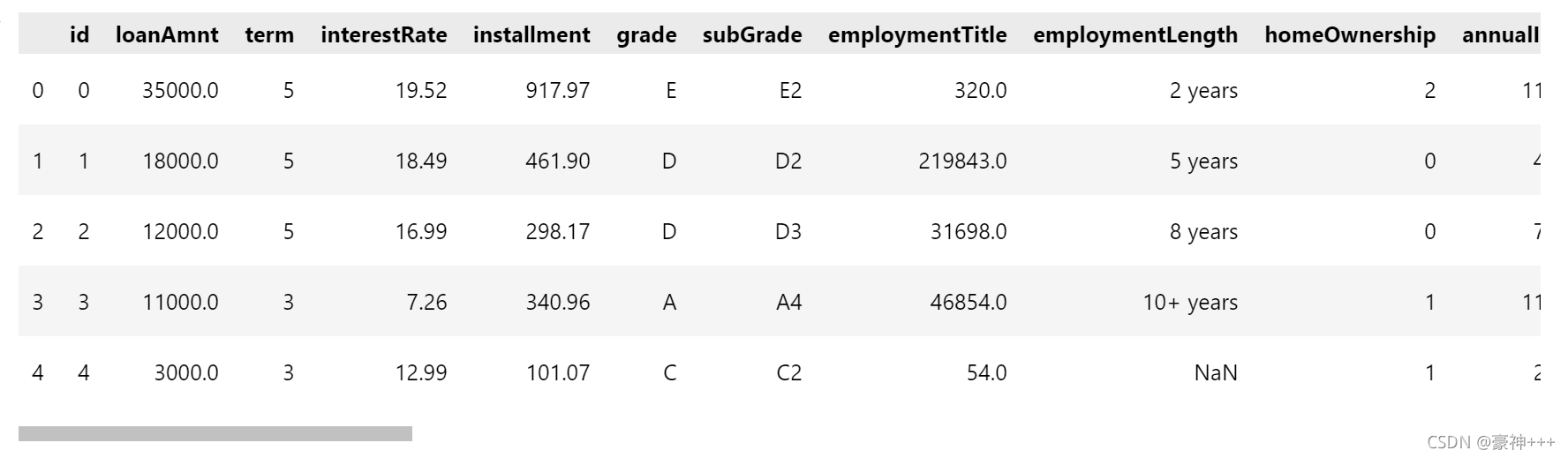
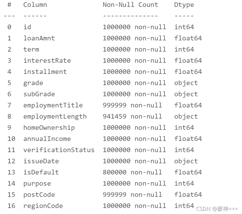
df.info()

在这里插入图片描述
缺失值处理

# 需要处理的列名
is_na_cols = [
    'employmentTitle', 'employmentLength', 'postCode', 'dti', 'pubRecBankruptcies',
    'revolUtil', 'title',] + [f'n{i}' for i in range(15)]

对缺失值用众数填充

# 对缺失值 用众数填充
for i in range(len(is_na_cols)):
    most_num = df[is_na_cols[i]].value_counts().index[0]
    df[is_na_cols[i]] = df[is_na_cols[i]].fillna(most_num)
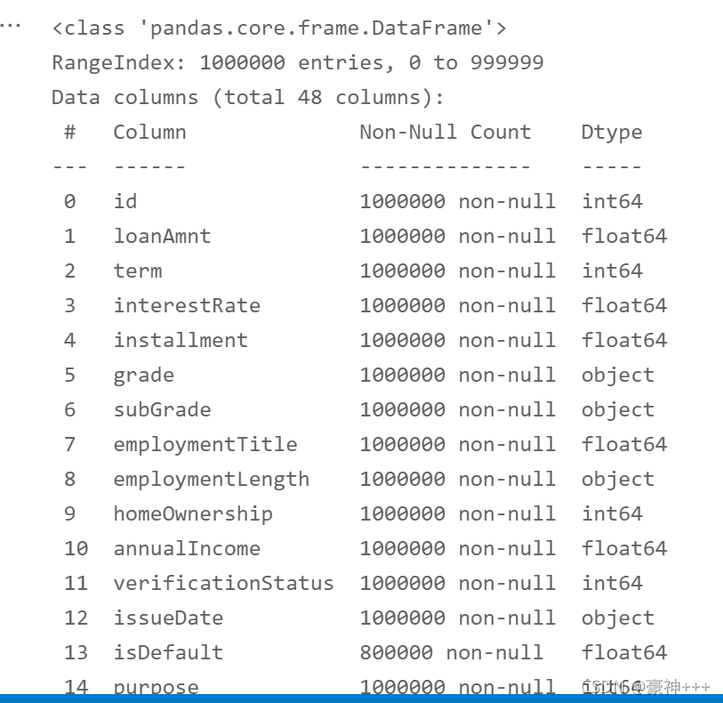
df.info()

在这里插入图片描述
分开训练集和测试集

df_train = df[df['train_test'] == 'train']
df_test = df[df['train_test'] == 'test']


del df_train['train_test']
del df_test['train_test']

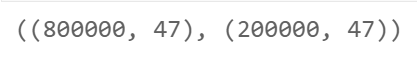
df_train.shape, df_test.shape

在这里插入图片描述
删除测试集的预测目标

del df_test['isDefault']

1.1.2数值型变量和非数值型变量的处理与分析

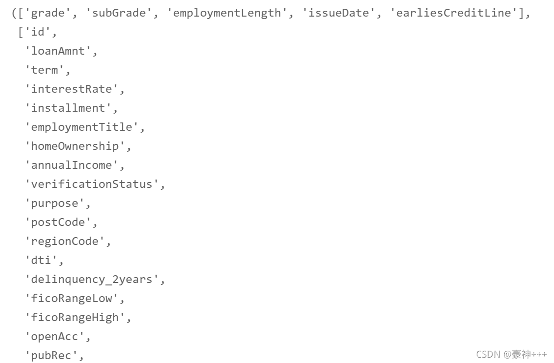
# 非数值型
non_numeric_cols = [
    'grade', 'subGrade', 'employmentLength', 'issueDate', 'earliesCreditLine'
]
# 数值型
numeric_cols = [
    x for x in df_test.columns if x not in non_numeric_cols + ['isDefault']
]
non_numeric_cols, numeric_cols

在这里插入图片描述

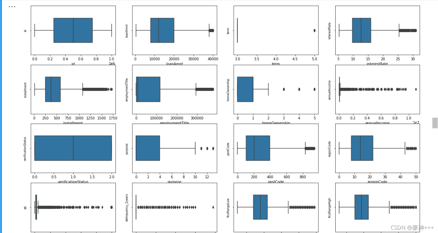
1.1.3数值型(numeric_cols)测试集与训练集分布

画箱式图可查看哪些列名是连续型和非连续型变量

# 画箱式图
column = numeric_cols # 列表头
fig = plt.figure(figsize=(20, 40))  # 指定绘图对象宽度和高度
for i in range(len(column)):
    plt.subplot(13, 4, i + 1)  # 13行3列子图
    sns.boxplot(df[column[i]], orient="v", width=0.5)  # 箱式图
    plt.ylabel(column[i], fontsize=8)
plt.show()

在这里插入图片描述

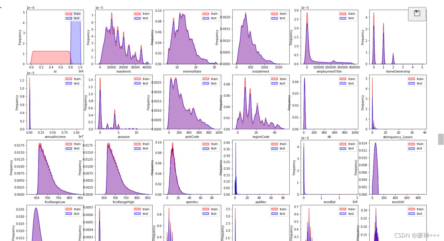
1.1.4取出数值连续性变量，查看数据分布

continuous_cols = [
    'id', 'loanAmnt', 'interestRate', 'installment', 'employmentTitle', 'homeOwnership',
    'annualIncome', 'purpose', 'postCode', 'regionCode', 'dti', 'delinquency_2years',
    'ficoRangeLow', 'ficoRangeHigh', 'openAcc', 'pubRec', 'revolBal', 'revolUtil','totalAcc',
    'title', 'n14'
] + [f'n{i}' for i in range(11)] 
non_continuous_cols = [
    x for x in numeric_cols if x not in continuous_cols
]

可视化正太分布，查看测试集与训练集的数据是否相同，相同可保留，差距会影响预测结果，就去除。

dist_cols = 6
dist_rows = len(df_test[continuous_cols].columns)
plt.figure(figsize=(4*dist_cols,4*dist_rows))

i=1
for col in df_test[continuous_cols].columns:
    ax=plt.subplot(dist_rows,dist_cols,i)
    ax = sns.kdeplot(df_train[continuous_cols][col], color="Red", shade=True)
    ax = sns.kdeplot(df_test[continuous_cols][col], color="Blue", shade=True)
    ax.set_xlabel(col)
    ax.set_ylabel("Frequency")
    ax = ax.legend(["train","test"])
    
    i+=1
plt.show()

在这里插入图片描述

画QQ图及正态分布图

QQ图：曲线越接近直线，越接近正态分布，预测效果更好。

train_cols = 6
train_rows = len(df[continuous_cols].columns)
plt.figure(figsize=(4*train_cols,4*train_rows))

i=0
for col in df[continuous_cols].columns:
    i+=1
    ax=plt.subplot(train_rows,train_cols,i)
    sns.distplot(df[continuous_cols][col],fit=stats.norm)
    i+=1
    ax=plt.subplot(train_rows,train_cols,i)
    res = stats.probplot(df[continuous_cols][col], plot=plt)
plt.show()

在这里插入图片描述
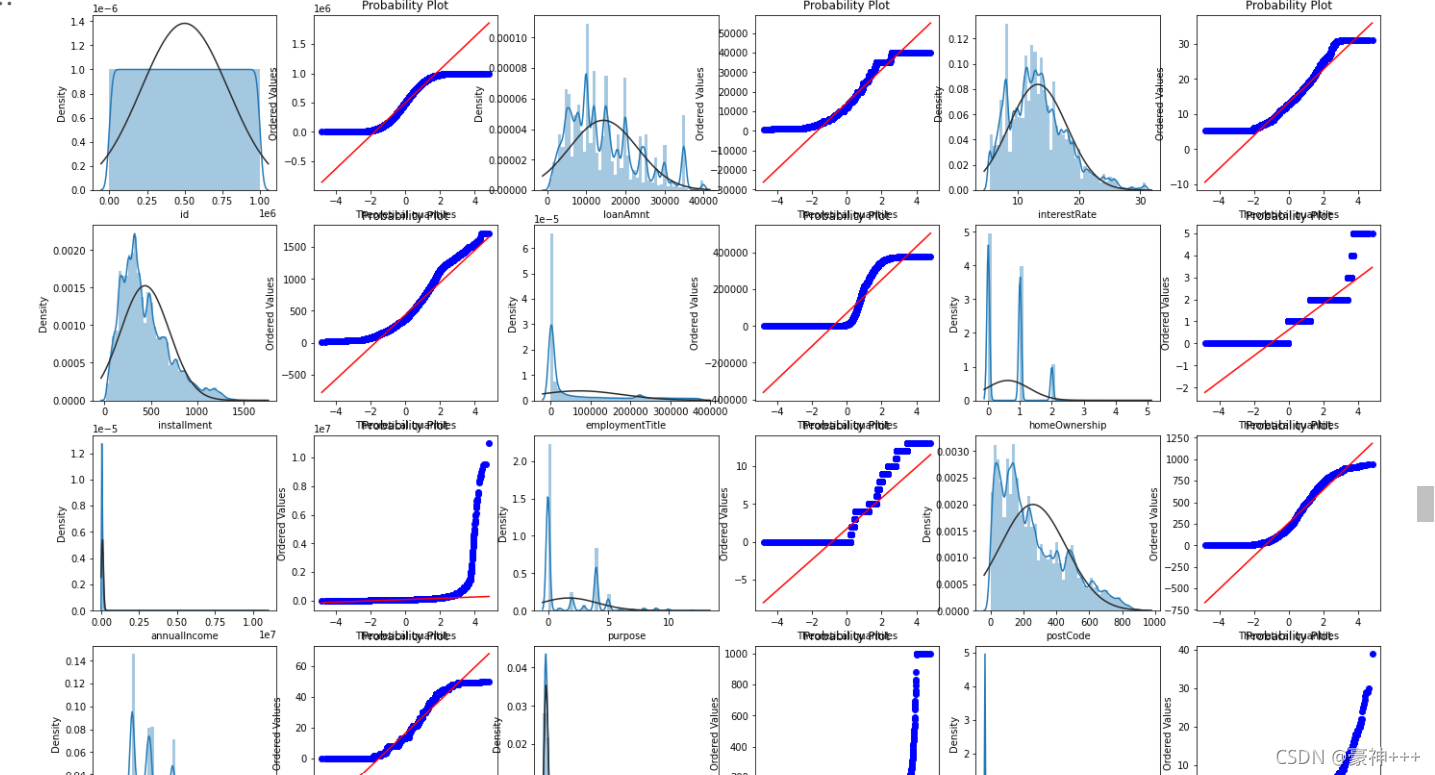
训练集的数据和测试集的数据分布差不多可以将他们整合到一起进行处理

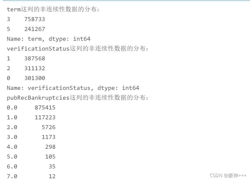
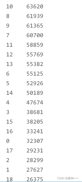
1.1.5查看数值非连续性型数据分布

for i in range(len(non_continuous_cols)):
    print("%s这列的非连续性数据的分布："%non_continuous_cols[i])
    print(df[non_continuous_cols[i]].value_counts())

在这里插入图片描述

1.1.6查看非数值型数据分布

for i in range(len(non_numeric_cols)):
    print("%s这列非数值型数据的分布：\n"%non_numeric_cols[i])
    print(df[non_numeric_cols[i]].value_counts())

在这里插入图片描述

2. 特征工程

2.1.1 数值非连续性型数据处理

policyCode字段

df['policyCode'].describe()

在这里插入图片描述

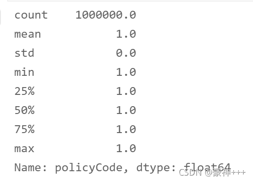
# 字段只有一个值，不用了
df.drop('policyCode',axis=1,inplace=True)

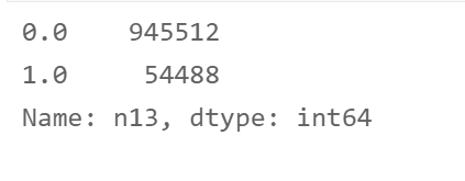
n13字段

df['n13'] = df['n13'].apply(lambda x: 1 if x not in [0] else x)
df['n13'].value_counts()

在这里插入图片描述

2.1.2 非数值型数据

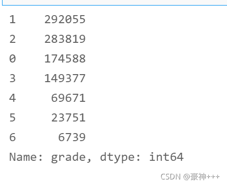
grade字段

# 非数值型编码
from sklearn.preprocessing import LabelEncoder
le = LabelEncoder()
df['grade'] = le.fit_transform(df['grade'])
df['grade'].value_counts()

在这里插入图片描述
2. subGrade字段

from sklearn.preprocessing import LabelEncoder
le = LabelEncoder()
df['subGrade'] = le.fit_transform(df['subGrade'])
df['subGrade'].value_counts()

在这里插入图片描述
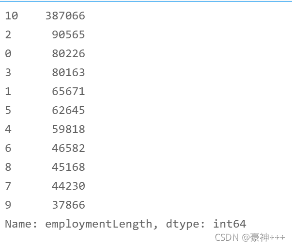
3. employmentLength字段

# 构造编码函数
def encoder(x):
    if x[:-5] == '10+ ':
        return 10
    elif x[:-5] == '< 1':
        return 0
    else:
        return int(x[0])
df['employmentLength'] = df['employmentLength'].apply(encoder)
df['employmentLength'].value_counts()

在这里插入图片描述
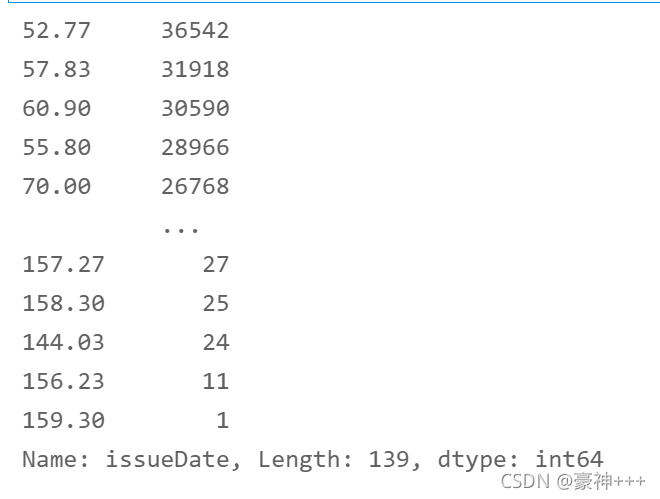
4. issueDate字段

计算离现在多少月就ok了

from datetime import datetime
def encoder1(x):
    x = str(x)
    now = datetime.strptime('2020-07-01','%Y-%m-%d')
    past = datetime.strptime(x,'%Y-%m-%d')
    period = now - past
    period = period.days
    return round(period / 30, 2)
df['issueDate'] = df['issueDate'].apply(encoder1)
df['issueDate'].value_counts()

在这里插入图片描述
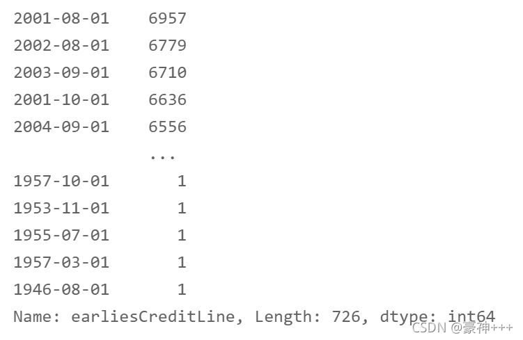
5. earliesCreditLine字段

def encoder2(x):
    if x[:3] == 'Jan':
        return x[-4:] + '-' + '01-01'
    if x[:3] == 'Feb':
        return x[-4:] + '-' + '02-01'
    if x[:3] == 'Mar':
        return x[-4:] + '-' + '03-01'
    if x[:3] == 'Apr':
        return x[-4:] + '-' + '04-01'
    if x[:3] == 'May':
        return x[-4:] + '-' + '05-01'
    if x[:3] == 'Jun':
        return x[-4:] + '-' + '06-01'
    if x[:3] == 'Jul':
        return x[-4:] + '-' + '07-01'
    if x[:3] == 'Aug':
        return x[-4:] + '-' + '08-01'
    if x[:3] == 'Sep':
        return x[-4:] + '-' + '09-01'
    if x[:3] == 'Oct':
        return x[-4:] + '-' + '10-01'
    if x[:3] == 'Nov':
        return x[-4:] + '-' + '11-01'
    if x[:3] == 'Dec':
        return x[-4:] + '-' + '12-01'
df['earliesCreditLine'] = df['earliesCreditLine'].apply(encoder2)
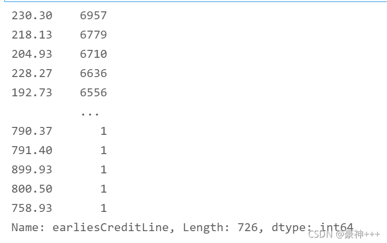
df['earliesCreditLine'].value_counts()

在这里插入图片描述

df['earliesCreditLine'] = df['earliesCreditLine'].apply(encoder1)
df['earliesCreditLine'].value_counts()

在这里插入图片描述

3. 保存文件

train = df[df['train_test'] == 'train']
test = df[df['train_test'] == 'test']

del test['isDefault']

del train['train_test']
del test['train_test']

train.to_csv('train_process.csv')
test.to_csv('test_process.csv')

4. 数据建模

4.1.1数据查看

# 数据处理
import numpy as np
import pandas as pd

# 数据可视化
import matplotlib.pyplot as plt

# 特征选择和编码
from sklearn.preprocessing import LabelEncoder

# 机器学习
from sklearn import model_selection, tree, preprocessing, metrics
from sklearn.ensemble import RandomForestClassifier, GradientBoostingClassifier
from sklearn.linear_model import LinearRegression, LogisticRegression, Ridge, Lasso, SGDClassifier
from sklearn.tree import DecisionTreeClassifier

# 网格搜索、随机搜索
import scipy.stats as st
from sklearn.model_selection import GridSearchCV
from sklearn.model_selection import RandomizedSearchCV

# 模型度量（分类）
from sklearn.metrics import precision_recall_fscore_support, roc_curve, auc

# 警告处理 
import warnings
warnings.filterwarnings('ignore')

# 在Jupyter上画图
%matplotlib inline

train = pd.read_csv('train_process.csv')
test = pd.read_csv('test_process.csv')
train.shape, test.shape

在这里插入图片描述

train.columns,test.columns

在这里插入图片描述

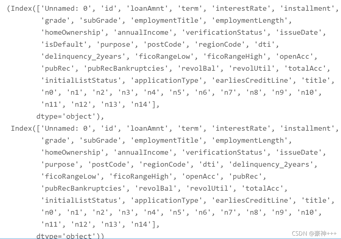
# 删除Unnamed: 0
del train['Unnamed: 0']
del test['Unnamed: 0']

## 为了正确评估模型性能，将数据划分为训练集和测试集，并在训练集上训练模型，在测试集上验证模型性能。
from sklearn.model_selection import train_test_split

## 选择其类别为0和1的样本 （不包括类别为2的样本）
data_target_part = train['isDefault']
data_features_part = train[[x for x in train.columns if x != 'isDefault' and 'id']]

## 测试集大小为20%， 80%/20%分
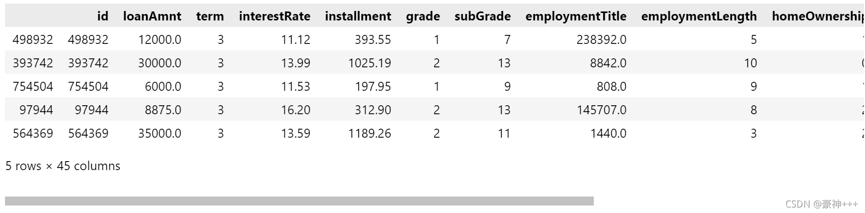
x_train, x_test, y_train, y_test = train_test_split(data_features_part, data_target_part, test_size = 0.2, random_state = 2020)

x_train.head()

在这里插入图片描述

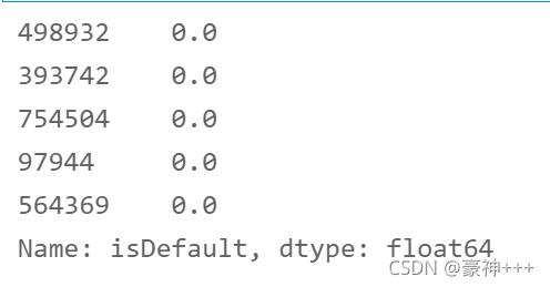
y_train.head()

在这里插入图片描述

4.1.1选择算法

以下是用到的算法.

Logistic Regression
Random Forest
Decision Tree
Gradient Boosted Trees

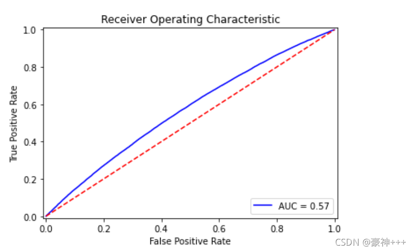
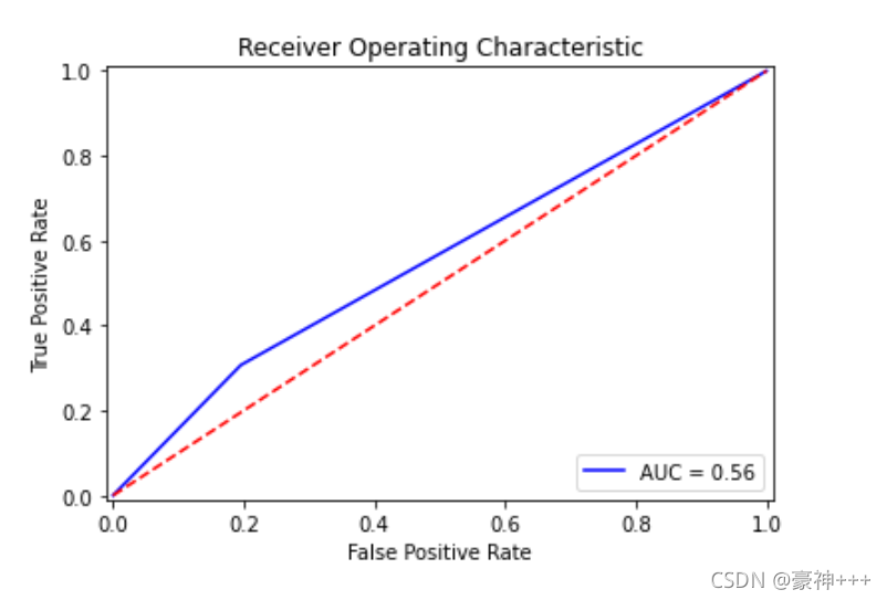
# 绘制AUC曲线
import time
def plot_roc_curve(y_test, preds):
    fpr, tpr, threshold = metrics.roc_curve(y_test, preds)
    roc_auc = metrics.auc(fpr, tpr)
    plt.title('Receiver Operating Characteristic')
    plt.plot(fpr, tpr, 'b', label = 'AUC = %0.2f' % roc_auc)
    plt.legend(loc = 'lower right')
    plt.plot([0, 1], [0, 1],'r--')
    plt.xlim([-0.01, 1.01])
    plt.ylim([-0.01, 1.01])
    plt.ylabel('True Positive Rate')
    plt.xlabel('False Positive Rate')
    plt.show()

# Logistic Regression
clf1 = LogisticRegression(solver='sag', max_iter=100, multi_class='multinomial')
clf1.fit(x_train, y_train)
## 在训练集和测试集上分布利用训练好的模型进行预测
train_predict = clf1.predict(x_train)
test_predict = clf1.predict(x_test)
from sklearn import metrics

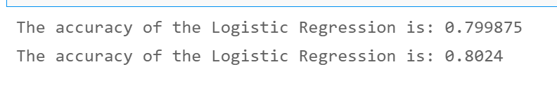
## 利用accuracy（准确度）【预测正确的样本数目占总预测样本数目的比例】评估模型效果
print('The accuracy of the Logistic Regression is:',metrics.accuracy_score(y_train,train_predict))
print('The accuracy of the Logistic Regression is:',metrics.accuracy_score(y_test,test_predict))

在这里插入图片描述

# 网格搜索
from sklearn.model_selection import GridSearchCV
param_grid = {
              'penalty': ['l2', 'l1'],
              'class_weight': [None, 'balanced'],
              'C': [0, 0.1, 0.5, 1],
                'intercept_scaling': [0.1, 0.5, 1]
             }

clf2 = LogisticRegression(solver='sag')
rfc = GridSearchCV(clf2, param_grid, scoring = 'neg_log_loss', cv=3, n_jobs=-1)
rfc.fit(x_train, y_train)
print(rfc.best_score_)
print(rfc.best_params_)

在这里插入图片描述

# Logistic Regression
clf1 = LogisticRegression(solver='sag', max_iter=100, penalty='l2', 
                          class_weight=None, C=0.1, intercept_scaling=0.1)
model = clf1.fit(x_train, y_train)
## 在训练集和测试集上分布利用训练好的模型进行预测
train_predict = clf1.predict(x_train)
test_predict = clf1.predict(x_test)
from sklearn import metrics

## 利用accuracy（准确度）【预测正确的样本数目占总预测样本数目的比例】评估模型效果
print('The accuracy of the Logistic Regression is:',metrics.accuracy_score(y_train,train_predict))
print('The accuracy of the Logistic Regression is:',metrics.accuracy_score(y_test,test_predict))

在这里插入图片描述

# 画图
plot_roc_curve(y_test, model.predict_proba(x_test)[:,1])

在这里插入图片描述

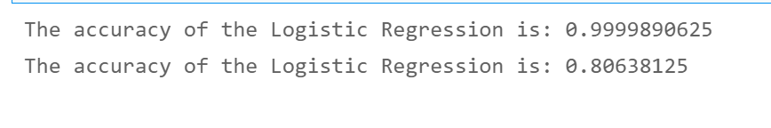
# Random Forest

clf1 = RandomForestClassifier()
clf1.fit(x_train, y_train)
## 在训练集和测试集上分布利用训练好的模型进行预测
train_predict = clf1.predict(x_train)
test_predict = clf1.predict(x_test)
from sklearn import metrics

## 利用accuracy（准确度）【预测正确的样本数目占总预测样本数目的比例】评估模型效果
print('The accuracy of the Logistic Regression is:',metrics.accuracy_score(y_train,train_predict))
print('The accuracy of the Logistic Regression is:',metrics.accuracy_score(y_test,test_predict))

在这里插入图片描述

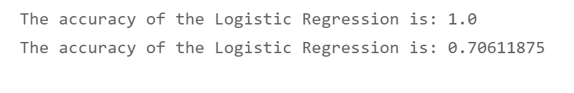
# 决策树
clf1 = DecisionTreeClassifier()
model = clf1.fit(x_train, y_train)
## 在训练集和测试集上分布利用训练好的模型进行预测
train_predict = clf1.predict(x_train)
test_predict = clf1.predict(x_test)
from sklearn import metrics

## 利用accuracy（准确度）【预测正确的样本数目占总预测样本数目的比例】评估模型效果
print('The accuracy of the Logistic Regression is:',metrics.accuracy_score(y_train,train_predict))
print('The accuracy of the Logistic Regression is:',metrics.accuracy_score(y_test,test_predict))

在这里插入图片描述

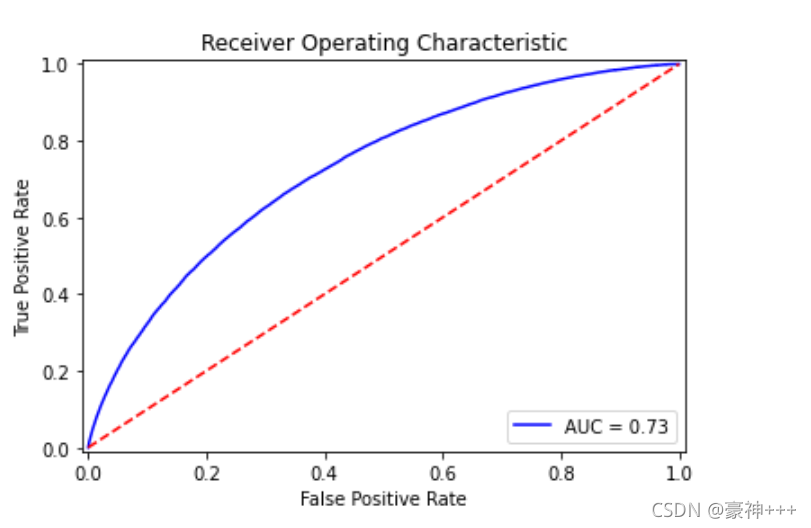
plot_roc_curve(y_test, model.predict_proba(x_test)[:,1])

在这里插入图片描述

# Gradient Boosting Trees

clf1 = GradientBoostingClassifier()
model = clf1.fit(x_train, y_train)
## 在训练集和测试集上分布利用训练好的模型进行预测
train_predict = clf1.predict(x_train)
test_predict = clf1.predict(x_test)
from sklearn import metrics

## 利用accuracy（准确度）【预测正确的样本数目占总预测样本数目的比例】评估模型效果
print('The accuracy of the Logistic Regression is:',metrics.accuracy_score(y_train,train_predict))
print('The accuracy of the Logistic Regression is:',metrics.accuracy_score(y_test,test_predict))

在这里插入图片描述

plot_roc_curve(y_test, model.predict_proba(x_test)[:,1])

在这里插入图片描述
代码演示结束

三、拓展

感兴趣的话还可以做一下特征融合、模型融合，做更好地特征工程使得模型AUC得分更高。

Haohao+++

关注

36
点赞
踩
156

收藏

觉得还不错? 一键收藏
30
评论
零基础入门金融风控-贷款违约预测-机器学习-数据分析

零基础入门金融风控-贷款违约预测一、赛题数据赛题以预测用户贷款是否违约为任务，数据集报名后可见并可下载，该数据来自某信贷平台的贷款记录，总数据量超过120w，包含47列变量信息，其中15列为匿名变量。为了保证比赛的公平性，将会从中抽取80万条作为训练集，20万条作为测试集A，20万条作为测试集B，同时会对employmentTitle、purpose、postCode和title等信息进行脱敏。字段表idFieldDescription1id为贷款清单分配的唯一信用证标
复制链接

扫一扫