ggplot2学习之6——geom_histogram画频率分布直方图频率加倍问题

说明

R语言的版本为4.0.2，IDE为Rstudio，版本为1.3.959。学习过程中参考了以下文章：
R语言ggplot2频率分布直方图小例子（简书）

1、geom_histogram函数说明

# 该函数用于绘制直方图，主要参数含义如下

# geom_histogram(
#   mapping = NULL, 		# 映射
#   data = NULL,			# 数据集
#   stat = "bin",			# 直方图类型
#   position = "stack",		# 位置
#   ...,					# 其它geom类函数的参数
#   binwidth = NULL,		# 直方图的间距
#   bins = NULL,			# 直方个数，和binwidth有类似效果，但设置逻辑不同
#   na.rm = FALSE,			# 逻辑参数，真值关闭缺值报错
#   orientation = NA,		# 方向
#   show.legend = NA,		# 逻辑参数，是否显示该图层的图例，NA为默认
#   inherit.aes = TRUE		# 逻辑参数，是否叠加本图层和默认的几何要素
# )

2、绘图举例

# 绘图数据
surge <- c(0.81,2.21,1.23,0.59,1.09,0.72,0.83,1.38,0.25,0.69,0.7,0.72,1.39,1.75,1.01,0.81,0.96,0.75,0.62,1.99,1.27,0.83,3.19,1.49,0.99)

# 设置..count..参数画计数直方图
GDPlot <- ggplot(surgeLing,aes(x = x, y =..count..)) +
  geom_histogram(aes(x = x, y =..count..),stat="bin",binwidth=1, boundary = 0)+
  geom_text(aes(label=as.character(round(..count..,2))),stat="bin",binwidth=1,boundary = 0,vjust=-0.5)

# 设置..density..频率分布直方图
GDPlot2 <- ggplot(surgeLing,aes(x = x, y =..density..)) +
  geom_histogram(aes(x = x, y =..density..),stat="bin",binwidth=1, boundary = 0)+
  geom_text(aes(label=as.character(round(..density..,2))),stat="bin",binwidth=1,boundary = 0,vjust=-0.5)
library("cowplot")
plot_grid(GDPlot, GDPlot2,nrow = 1, ncol = 2 )

3、画频率分布直方图频率加倍

当使用bins参数或者binwidth参数，对频率分布直方图进行调整的时候，发现如果不指定binwidth参数为1，则频率会加倍，有可能频率出现大于1的情况，这显然不合理。

# 绘图数据
 surge <- c(0.81,2.21,1.23,0.59,1.09,0.72,0.83,1.38,0.25,0.69,0.7,0.72,1.39,1.75,1.01,0.81,0.96,0.75,0.62,1.99,1.27,0.83,3.19,1.49,0.99)

# 画间距为1的频率分布直方图，正常显示
GDPlot <- ggplot(surgeLing,aes(x = x, y =..density..)) +
  geom_histogram(aes(x = x, y =..density..),stat="bin",binwidth=1, boundary = 0)+
  geom_text(aes(label=as.character(round(..density..,2))),stat="bin",binwidth=1,boundary = 0,vjust=-0.5)

# 画间距为0.5的频率分布直方图，频率被加倍了
GDPlot2 <- ggplot(surgeLing,aes(x = x, y =..density..)) +
  geom_histogram(aes(x = x, y =..density..),stat="bin",binwidth=0.5, boundary = 0)+
  geom_text(aes(label=as.character(round(..density..,2))),stat="bin",binwidth=0.5,boundary = 0,vjust=-0.5)
library("cowplot")
plot_grid(GDPlot, GDPlot2,nrow = 1, ncol = 2 )

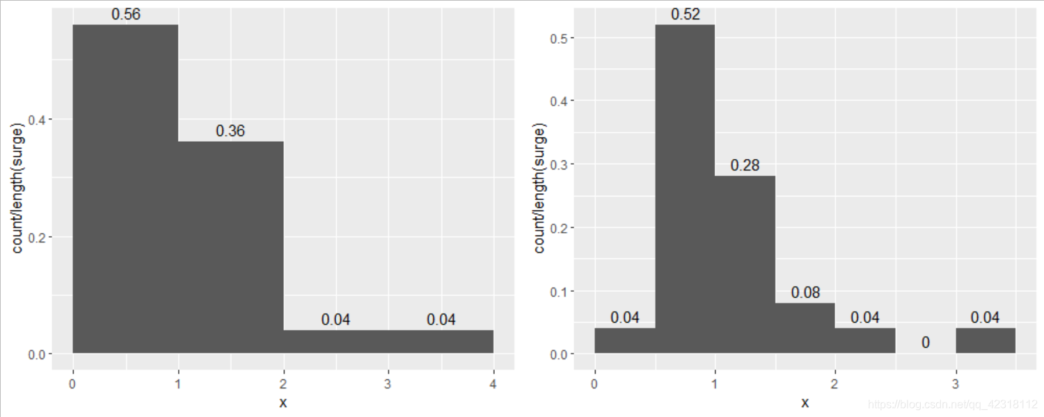
4、解决办法

经过测试，发现使用计数直方图绘图是，改变间距，不会改变各个区间点据的数值，索性自己吧计数直方图改成频率分布直方图，只需在y轴…count…后除以数据长度即可

# 绘图数据
 surge <- c(0.81,2.21,1.23,0.59,1.09,0.72,0.83,1.38,0.25,0.69,0.7,0.72,1.39,1.75,1.01,0.81,0.96,0.75,0.62,1.99,1.27,0.83,3.19,1.49,0.99)

# 间距为1时显示正常
GDPlot <- ggplot(surgeLing,aes(x = x, y =..count../length(surge))) +
  geom_histogram(aes(x = x, y =..count../length(surge)),stat="bin",binwidth=1, boundary = 0)+
  geom_text(aes(label=as.character(round(..count../length(surge),2))),stat="bin",binwidth=1,boundary = 0,vjust=-0.5)

# 间距为0.5时也显示正常
GDPlot2 <- ggplot(surgeLing,aes(x = x, y =..count../length(surge))) +
  geom_histogram(aes(x = x, y =..count../length(surge)),stat="bin",binwidth=0.5, boundary = 0)+
  geom_text(aes(label=as.character(round(..count../length(surge),2))),stat="bin",binwidth=0.5,boundary = 0,vjust=-0.5)
library("cowplot")
plot_grid(GDPlot, GDPlot2,nrow = 1, ncol = 2 )

# 问题解决