fmriprep对应outputs文件的记录

前言

记录对生成的html结果文档的简单介绍；参考：
fmriprep官网
Andy’s brainbook
示例：

1.summary

“摘要”包含有关结构和功能图像数量、用于规范化的模板以及是否运行 FreeSurfer 的详细信息。

2.Anatomical

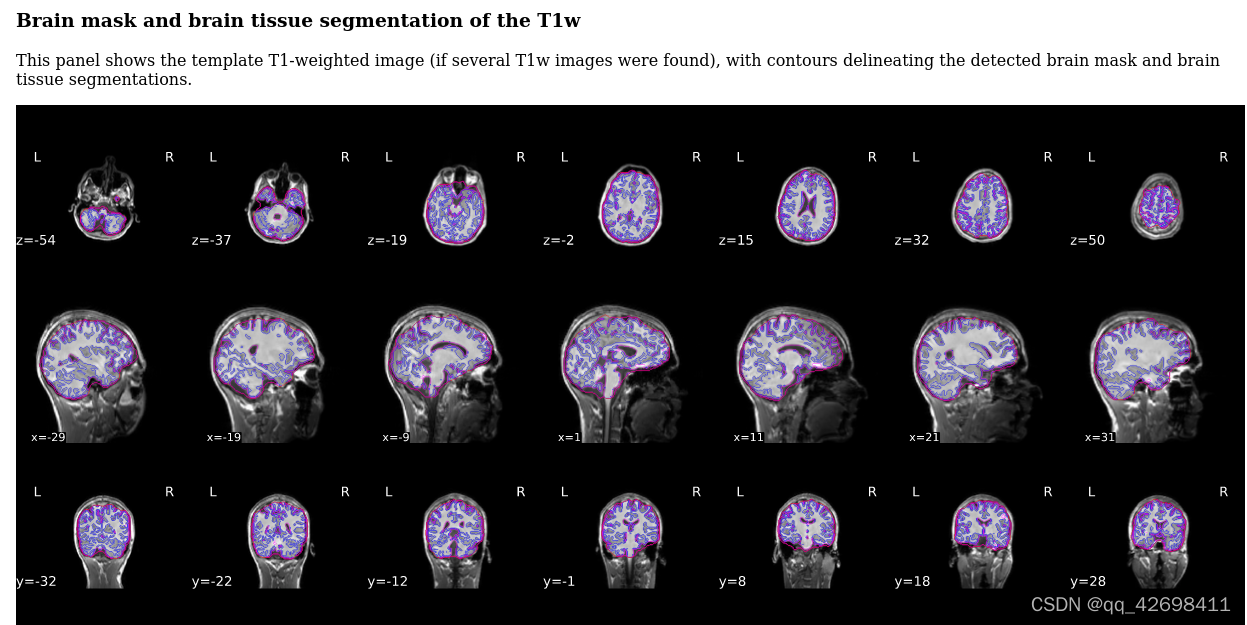
structural vs functional：结构是指对大脑结构进行成像，即其解剖特性；功能性——大脑功能，即与特定任务相关的区域。
1）white vs pial surface：白色表面勾勒出白色和灰质之间的边界，用蓝线表示，而 pial——灰质和脑脊液之间的边界，用洋红线表示；因此，我们使用白色和软脑膜表面分别量化白质体积和灰质体积。
所有图形都有对应于三个解剖平面的三个“行”：横向、矢状和冠状
2）将解剖图像标准化为模板以来回 GIF 的形式显示。 确保不仅要检查大脑轮廓之间的对齐，注意还要检查脑室等内部结构。

3.Functional
1)使用 GIF 来显示功能图像和解剖图像之间的对齐;
2)解剖成分校正 (anatCompCor) 的掩模轮廓;功能组件校正（funcCompCor）,使用这些体素生成白质、CSF、组合白质和 CSF 以及时间标准偏差的 compCor 曲线，这些曲线显示了由不同数量的分量解释的方差量。

Some of the estimated confounds are plotted with a “carpet” visualization of the BOLD time series：

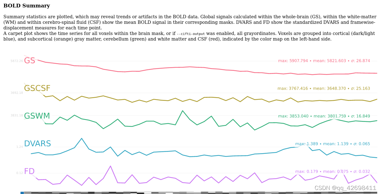
The figure shows on top several confounds estimated for the BOLD series: global signals (‘GlobalSignal’, ‘WM’, ‘GM’), standardized DVARS (‘stdDVARS’), and framewise-displacement (‘FramewiseDisplacement’). At the bottom, a ‘carpetplot’ summarizing the BOLD series. The color-map on the left-side of the carpetplot denotes signals located in cortical gray matter regions (blue), subcortical gray matter (orange), cerebellum (green) and the union of white-matter and CSF compartments (red)
该图显示了为 BOLD 系列估计的几个混淆：
全局信号（“GlobalSignal”、“WM”、“GM”）
标准化 DVARS（“stdDVARS”）
逐帧位移（“FramewiseDisplacement”）。
运动的变化往往与全局信号的​​变化相关，是否在模型中包含任何这些回归变量取决于做实验者自身。一般来说，DVARS 和 FD 是解释由运动伪影引起的信号的好方法。

地毯图左侧的彩色图表示位于皮质灰质区域（蓝色）、皮质下灰质（橙色）、小脑（绿色）以及白质和 CSF 隔室（红色）的结合处的信号（ The color-map on the left-side of the carpetplot denotes signals located in cortical gray matter regions (blue), subcortical gray matter (orange), cerebellum (green) and the union of white-matter and CSF compartments (red)）运动的任何突然变化都可能反映在该时间点整个列的均匀变化中。

The figure displays the cumulative variance explained by components for each of four CompCor decompositions (left to right: anatomical CSF mask, anatomical white matter mask, anatomical combined mask, temporal). The number of components is plotted on the abscissa and the cumulative variance explained on the ordinate. Dotted lines indicate the minimum number of components necessary to explain 50%, 70%, and 90% of the variance in the nuisance mask. By default, only the components that explain the top 50% of the variance are saved.（参考翻译：报告包括由每个组件解释的累积方差图，按奇异值降序排列。该图显示了由四个 CompCor 分解中的每一个的组件解释的累积方差（从左到右：解剖 CSF 掩模、解剖白质掩模、解剖组合掩模、时间）。组件的数量绘制在横坐标上，累积方差解释在纵坐标上。虚线表示解释 50%、70% 和 90% 的 nuisance mask方差所需的最少components。默认情况下，仅保存解释前 50% 方差的分量。）

混淆回归变量之间的相关图。 这可用于指导混淆模型的选择或评估组织特异性回归因子与全局信号的相关程度。
左侧面板将所选混淆时间序列之间的相关矩阵显示为热图（shows correlations between the different nuisance regressors）。 注意对角线附近的零相关块； 这些对应于每个 CompCor 分解。 右侧面板显示了选定的混杂时间序列与整个大脑计算的平均全局信号的相关性； 显示的回归量是与全局信号相关性最大的回归量。 此信息可用于诊断部分体积效应。
The left-hand panel shows the matrix of correlations among selected confound time series as a heat-map. Note the zero-correlation blocks near the diagonal; these correspond to each CompCor decomposition. The right-hand panel displays the correlation of selected confound time series with the mean global signal computed across the whole brain; the regressors shown are those with greatest correlation with the global signal. This information can be used to diagnose partial volume effects