数据科学包16、matplotlib的实例

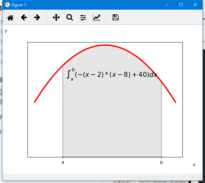
1.函数积分图

# 函数积分图
import numpy as np
import matplotlib.pyplot as plt
from matplotlib.patches import Polygon

def func(x):
    return -(x-2)*(x-8) + 40
# 将0-10区间等分50份 返回array数组
x = np.linspace(0,10)

y = func(x)
# 构造绘图窗口与坐标轴
fig, ax = plt.subplots()
ax.plot(x,y,'r',linewidth=3)

a = 2
b = 9
# 对x、y轴的坐标刻度取消，参数为列表，可选
ax.set_xticks([a,b])
ax.set_yticks([])
# 设置标签，并且将标签写成数学符号
ax.set_xticklabels([r'$a$',r'$b$'])
# 设置x、y---figtext
plt.figtext(0.95,0.05,'$x$')
plt.figtext(0.01,0.95,'$y$')

# 画多边形
ix = np.linspace(a,b)
iy = func(ix)
ixy = zip(ix,iy)
verts = [(a,0)] + list(ixy) + [(b,0)]
# 调用Polygon画多边形
poly = Polygon(verts,facecolor='0.9',edgecolor='0.5')

ax.add_patch(poly)


# 添加数学公式
x_math = (a+b)*0.5
y_math = 35
# horizontalalignment='center'控制公式自动中间对齐
ax.text(x_math,y_math,r'$\int_a^b(-(x-2)*(x-8) + 40)dx$',fontsize=15,horizontalalignment='center')

plt.ylim(bottom=0)
plt.show()

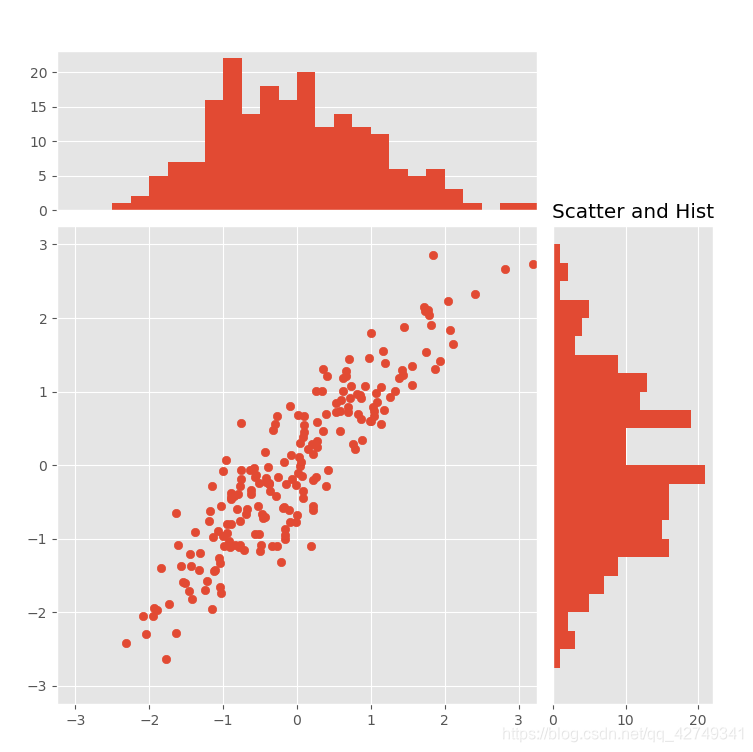
2.散点图-条形图结合

# 散点-条形图
import numpy as np
import matplotlib.pyplot as plt

# 图形为了美观直接使用'ggplot'风格
plt.style.use('ggplot')

# 从标准正态分布中返回多个样本值
x = np.random.randn(200)
y = x + np.random.randn(200)*0.5

margin_border = 0.1
width = 0.6
margin_between = 0.02
height = 0.2

# 第一个子图的位置信息
left_s = margin_border
bottom_s = margin_border
height_s = width
width_s = width

# 上面子图的位置信息
left_x = margin_border
bottom_x = margin_border + width + margin_between
height_x = height
width_x = width

# 右边子图的位置信息
left_y = margin_border + width + margin_between
bottom_y = margin_border
height_y = width
width_y = height

plt.figure(1,figsize=(8,8))

rect_s =[left_s,bottom_s,width_s,height_s]
rect_x =[left_x,bottom_x,width_x,height_x]
rect_y =[left_y,bottom_y,width_y,height_y]

# 生成三个图形
axScatter = plt.axes(rect_s)
axHisX = plt.axes(rect_x)
axHisY = plt.axes(rect_y)

# 去掉重复坐标轴
axHisX.set_xticks([])
axHisY.set_yticks([])

# 画散点图,x,y默认为20，y正负控制相关性
axScatter.scatter(x,y)

bin_width = 0.25
xymax = np.max([np.max(np.fabs(x)),np.max(np.fabs(y))])
lim = int(xymax/bin_width + 1) * bin_width

# 调整坐标轴刻度
axScatter.set_xlim(-lim,lim)
axScatter.set_ylim(-lim,lim)

# 画直方图
bins = np.arange(-lim,lim+bin_width,bin_width)

axHisX.hist(x,bins = bins)
axHisY.hist(y,bins = bins,orientation='horizontal')

# 调整两个子图的坐标轴刻度
axHisX.set_xlim(axScatter.get_xlim())
axHisY.set_ylim(axScatter.get_ylim())

# 添加标题
plt.title('Scatter and Hist',)

plt.show()

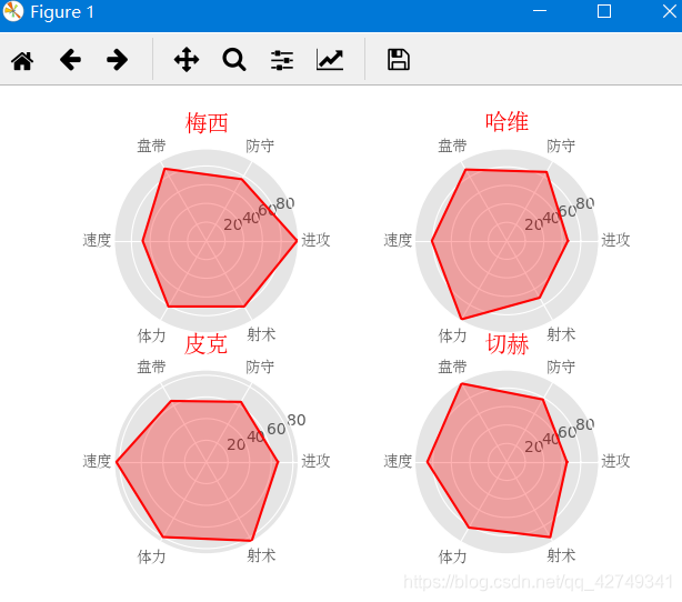
3.球员能力图

# 球员能力图
import numpy as np
import matplotlib.pyplot as plt
# 专门管理字体的类
from matplotlib.font_manager import FontProperties

plt.style.use('ggplot')
# 定义字体
font = FontProperties(fname=r'c:\windows\fonts\simsun.ttc',size=10)
# 能力标签
ability_size = 6
ability_label = ['进攻','防守','盘带','速度','体力','射术']
# 生成4个子图
ax1 = plt.subplot(221,projection='polar')
ax2 = plt.subplot(222,projection='polar')
ax3 = plt.subplot(223,projection='polar')
ax4 = plt.subplot(224,projection='polar')

# 随机生成球员能力
player = {
    'M':np.random.randint(size=ability_size,low=60,high=99),
    'H':np.random.randint(size=ability_size,low=60,high=99),
    'P':np.random.randint(size=ability_size,low=60,high=99),
    'Q':np.random.randint(size=ability_size,low=60,high=99),
}
# 角度值,首尾相接共7个
theta = np.linspace(0,2*np.pi,6,endpoint=False)
theta = np.append(theta,theta[0])
player['M'] = np.append(player['M'],player['M'][0])
# 画图
ax1.plot(theta,player['M'],'r')
# 填充颜色
ax1.fill(theta,player['M'],'r',alpha=0.3)
# 重新生成极坐标 与能力对应
ax1.set_xticks(theta)
# 设置标签,此时，字体并没有正确的显示出来，matplotlib不知道用什么字体读取，需要显式的设置
ax1.set_xticklabels(ability_label,y=0.05,fontproperties=font)
# 添加标签
ax1.set_title('梅西',fontproperties=font,color='r',size=15)

player['H'] = np.append(player['H'],player['H'][0])
ax2.plot(theta,player['H'],'r')
ax2.fill(theta,player['H'],'r',alpha=0.3)
ax2.set_xticks(theta)
ax2.set_xticklabels(ability_label,y=0.05,fontproperties=font)
ax2.set_title('哈维',fontproperties=font,color='r',size=15)

player['P'] = np.append(player['P'],player['P'][0])
ax3.plot(theta,player['P'],'r')
ax3.fill(theta,player['P'],'r',alpha=0.3)
ax3.set_xticks(theta)
ax3.set_xticklabels(ability_label,y=0.05,fontproperties=font)
ax3.set_title('皮克',fontproperties=font,color='r',size=15)

player['Q'] = np.append(player['Q'],player['Q'][0])
ax4.plot(theta,player['Q'],'r')
ax4.fill(theta,player['Q'],'r',alpha=0.3)
ax4.set_xticks(theta)
ax4.set_xticklabels(ability_label,y=0.05,fontproperties=font)
ax4.set_title('切赫',fontproperties=font,color='r',size=15)

plt.show()