【Machine Learning】6. Linear Regression using Scikit-Learn

一藏过往

已于 2023-12-22 20:38:22 修改

阅读量977

点赞数 20

CC 4.0 BY-SA版权

分类专栏： Machine Learning 文章标签：机器学习线性回归 scikit-learn

于 2023-12-22 20:27:52 首次发布

本文链接：https://blog.csdn.net/qq_42887833/article/details/135159713

Machine Learning 专栏收录该内容

8 篇文章

订阅专栏

本文介绍了如何使用Scikit-Learn库中的SGDRegressor进行梯度下降回归，并通过实例演示了单特征和多特征线性回归，包括数据预处理、模型创建、参数查看及预测。同时介绍了闭式解线性回归在简单数据集上的应用。

摘要生成于 C知道，由 DeepSeek-R1 满血版支持，前往体验 >

1 前言

Scikit-learn 是一个热门且可靠的机器学习库，拥有各种算法，同时也是用于 ML 可视化、预处理、模型拟合、选择和评估的工具。
对于前几篇文章的线性回归和梯度下降等，可以直接调用现有的库进行运算。
了解Scikit-Learn

2 使用Scikit-learn实例

下面有三个实例，2.1中是一个 SGDRegressor实例，2.2中是两个Linear Regression的实例。

2.0 导入库

import numpy as np
np.set_printoptions(precision=2)
# 从库中导入回归对象
from sklearn.linear_model import LinearRegression, SGDRegressor
# 从库中导入数据标准化类
from sklearn.preprocessing import StandardScaler
from lab_utils_multi import  load_house_data
import matplotlib.pyplot as plt
dlblue = '#0096ff'; dlorange = '#FF9300'; dldarkred='#C00000'; dlmagenta='#FF40FF'; dlpurple='#7030A0'; 
plt.style.use('./deeplearning.mplstyle')

2.1 SGDRegressor

Scikit-learn has a gradient descent regression model sklearn.linear_model.SGDRegressor. Like your previous implementation of gradient descent, this model performs best with normalized inputs. sklearn.preprocessing.StandardScaler will perform z-score normalization as in a previous lab. Here it is referred to as ‘standard score’.

Scikit-learn有一个梯度下降回归模型sklearn.linear_model.SGDRegressor。与之前的梯度下降实现一样，该模型在标准化输入时表现最好，standardscaler需要像之前的实验一样执行z-score归一化。Scikit-learn也提供了归一化的库 sklearn.preprocessing.StandardScaler 。

Load the data set （导入数据集）

X_train, y_train = load_house_data()
X_features = ['size(sqft)','bedrooms','floors','age']

Scale/normalize the training data（特征缩放、归一化）

scaler = StandardScaler() # 创建一个用来归一化的对象
X_norm = scaler.fit_transform(X_train) # 归一化数据集X_train
print(f"Peak to Peak range by column in Raw        X:{np.ptp(X_train,axis=0)}")   
print(f"Peak to Peak range by column in Normalized X:{np.ptp(X_norm,axis=0)}")

np.ptp(x,axis=0/1) 的用法是求出纵轴/横轴的最大值减去最小值，详见numpy.ptp

Create and fit the regression model (创建回归模型)

创建SGDRegressor对象（使用梯度下降方法拟合）后使用fit函数拟合数据

sgdr = SGDRegressor(max_iter=1000) # 创建SGDRegressor对象
sgdr.fit(X_norm, y_train)
print(sgdr)
print(f"number of iterations completed: {sgdr.n_iter_}, number of weight updates: {sgdr.t_}")

""" 输出结果
SGDRegressor()
number of iterations completed: 110, number of weight updates: 10891.0
"""

View parameters （查看模型参数）

Note, the parameters are associated with the normalized input data. The fit parameters are very close to those found in the previous lab with this data.

b_norm = sgdr.intercept_
w_norm = sgdr.coef_
print(f"model parameters:                   w: {w_norm}, b:{b_norm}")
print(f"model parameters from previous lab: w: [110.56 -21.27 -32.71 -37.97], b: 363.16")

""" 输出结果 
model parameters:                   w: [109.88 -20.92 -32.31 -38.1 ], b:[363.16]
model parameters from previous lab: w: [110.56 -21.27 -32.71 -37.97], b: 363.16
"""

Make predictions（预测）

Predict the targets of the training data. Use both the predict routine and compute using $w$ and $b$ .

# make a prediction using sgdr.predict()
y_pred_sgd = sgdr.predict(X_norm)
# make a prediction using w,b. 
y_pred = np.dot(X_norm, w_norm) + b_norm  
print(f"prediction using np.dot() and sgdr.predict match: {(y_pred == y_pred_sgd).all()}")

print(f"Prediction on training set:\n{y_pred[:4]}" )
print(f"Target values \n{y_train[:4]}")

"""输出结果
prediction using np.dot() and sgdr.predict match: True
Prediction on training set:
[295.17 485.86 389.65 492.02]
Target values 
[300.  509.8 394.  540. ]
"""

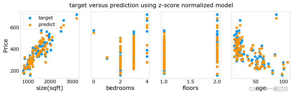
Plot Results

Let’s plot the predictions versus the target values.

# plot predictions and targets vs original features    
fig,ax=plt.subplots(1,4,figsize=(12,3),sharey=True)
for i in range(len(ax)):
    ax[i].scatter(X_train[:,i],y_train, label = 'target')
    ax[i].set_xlabel(X_features[i])
    ax[i].scatter(X_train[:,i],y_pred,color=dlorange, label = 'predict')
ax[0].set_ylabel("Price"); ax[0].legend();
fig.suptitle("target versus prediction using z-score normalized model")
plt.show()

请添加图片描述

2.2 Linear Regression, closed-form solution

First example（单特征回归）

Scikit-learn has the linear regression model which implements a closed-form linear regression.

Let’s use the data from the early labs - a house with 1000 square feet sold for $300,000 and a house with 2000 square feet sold for $500,000.

Size (1000 sqft)	Price (1000s of dollars)
1	300
2	500

Load the data set

X_train = np.array([1.0, 2.0])   #features
y_train = np.array([300, 500])   #target value

Create and fit the model（创建模型）

The code below performs regression using scikit-learn.
The first step creates a regression object.
The second step utilizes one of the methods associated with the object, fit. This performs regression, fitting the parameters to the input data. The toolkit expects a two-dimensional X matrix.

创建LinearRegression（这里是与2.1最大的区别，使用的拟合方式不同）对象后使用fit函数拟合数据

linear_model = LinearRegression()
#X must be a 2-D Matrix
linear_model.fit(X_train.reshape(-1, 1), y_train) 
""" 结果
LinearRegression()
"""

View Parameters （查看参数）

The $\mathbf{w}$ and $\mathbf{b}$ parameters are referred to as ‘coefficients’ and ‘intercept’ in scikit-learn.

查看模型参数intercept_和coef_

b = linear_model.intercept_
w = linear_model.coef_
print(f"w = {w:}, b = {b:0.2f}")
print(f"'manual' prediction: f_wb = wx+b : {1200*w + b}")

"""结果
w = [200.], b = 100.00
'manual' prediction: f_wb = wx+b : [240100.]
"""

Make Predictions（预测）

Calling the predict function generates predictions.

y_pred = linear_model.predict(X_train.reshape(-1, 1))

print("Prediction on training set:", y_pred)

X_test = np.array([[1200]])
print(f"Prediction for 1200 sqft house: ${linear_model.predict(X_test)[0]:0.2f}")

"""结果
Prediction on training set: [300. 500.]
Prediction for 1200 sqft house: $240100.00
"""

Second Example （多特征回归）

The second example is from an earlier lab with multiple features. The final parameter values and predictions are very close to the results from the un-normalized ‘long-run’ from that lab. That un-normalized run took hours to produce results, while this is nearly instantaneous. The closed-form solution work well on smaller data sets such as these but can be computationally demanding on larger data sets.

The closed-form solution does not require normalization.

基本过程跟上一个例子一样，只是变成多特征回归。

# load the dataset
X_train, y_train = load_house_data()
X_features = ['size(sqft)','bedrooms','floors','age']

linear_model = LinearRegression()
linear_model.fit(X_train, y_train) 
"""结果
LinearRegression()
"""

b = linear_model.intercept_
w = linear_model.coef_
print(f"w = {w:}, b = {b:0.2f}")
"""结果
w = [  0.27 -32.62 -67.25  -1.47], b = 220.42
"""

print(f"Prediction on training set:\n {linear_model.predict(X_train)[:4]}" )
print(f"prediction using w,b:\n {(X_train @ w + b)[:4]}")
print(f"Target values \n {y_train[:4]}")

x_house = np.array([1200, 3,1, 40]).reshape(-1,4)
x_house_predict = linear_model.predict(x_house)[0]
print(f" predicted price of a house with 1200 sqft, 3 bedrooms, 1 floor, 40 years old = ${x_house_predict*1000:0.2f}")

"""结果
Prediction on training set:
 [295.18 485.98 389.52 492.15]
prediction using w,b:
 [295.18 485.98 389.52 492.15]
Target values 
 [300.  509.8 394.  540. ]
 predicted price of a house with 1200 sqft, 3 bedrooms, 1 floor, 40 years old = $318709.09
 """