


Lecture 01
Preface
Data source:https://b23.tv/av5625356/p1
1. Some Reference Material
R Cookbook: http://www.cookbook-r.com/
R in Action: http://www.amazon.com/R-Action-Robert-Kabacoff/dp/1935182390
ggplot2: Elegant Graphics for Data Analysis (Use R!): http://www.amazon.com/ggplot2-
Elegant-Graphics-Data-Analysis/dp/0387981403
Advanced R: http://adv-r.had.co.nz/ & http://www.amazon.com/Advanced-Chapman-Hall-CRC-Series/dp/1466586966
Install Studio
http://blog.sina.com.cn/s/blog_c685f68e0102wc50.html

2. Installing and Loading Package
Installing: install.packages(’ggplot2’)
**Loading: **library(ggplot2)
Updating: update.packages()
3. R language basics
Create a vector: v = c(1,4,4,3,2,2,3) or w = c(”apple”,”banana”,”orange”)
Return certain elements: v[c(2,3,4)] or v[2:4] or v[c(2,4,3)]
Delete certain element: v = v[-2] or v = v[-2:-4]
Extract elements: v[v<3]
Find elements: which(v==3) Note: the returns are the indices of elements
> v=c(1,4,4,3,2,2,3)
> v[c(2,3,4)]      #第2,3,4个数
[1] 4 4 3

> v[2:4]      #第2到第4个数
[1] 4 4 3

> v[2:5]      #第2到第5个数
[1] 4 4 3 2

> v[2,4,3]        #error
Error in v[2, 4, 3] : incorrect number of dimensions

> v[c(2,4,3)]      #第2,4,3个数
[1] 4 3 4

> v[-2]      #删除第2个数
[1] 1 4 3 2 2 3

> v[-2:-4]    #删除第2到第4个数
[1] 1 2 2 3

> v[v<3]
[1] 1 2 2      #小于3的数

> which(v==3)
[1] 4 7      #找到值为3的数的位置,即第4个数,第7个数等于3

> which.max(v)      #返回向量里的第一个最大值
[1] 2
> which.min(v)      #返回向量里的第一个最小值的位置
[1] 1
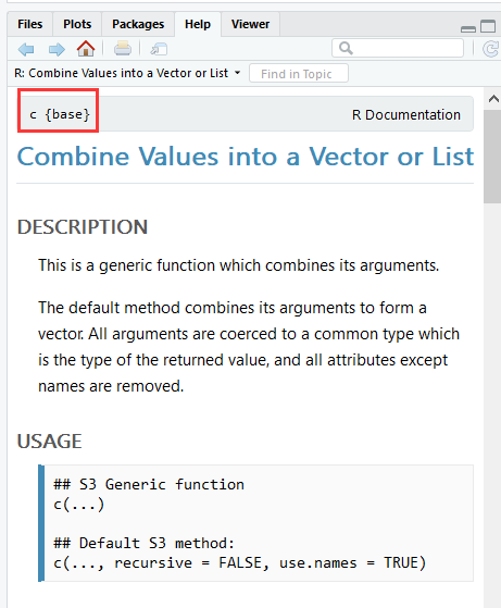
> ?c
4. Numbers
Random Number: a = runif(3, min=0, max=100)
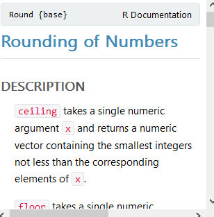
Rounding of Numbers: floor(a) or ceiling(a) or round(a,4)
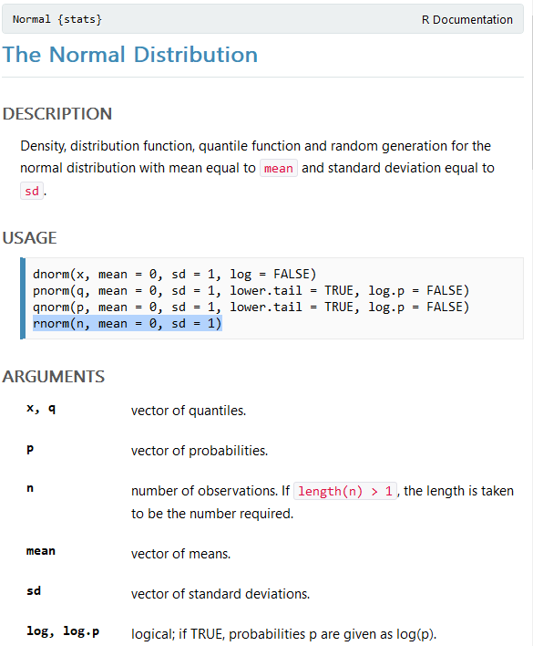
Random Numbers from Other Distributions: rnorm(), rexp(), rbinom(),
rgeom(), rnbinom() and so on.
Repeatable Random Numbers: set.seed()
#如何处理随机数
> set.seed(250)
> a = runif(3, min=0, max=100)
> set.seed(250)
> a
[1] 26.54018 77.90907 16.90836
> floor(a)      #取整
[1] 26 77 16
> ceiling(a)
[1] 27 78 17
> round(a,4)      #对向量a保留4位小数
[1] 26.5402 77.9091 16.9084
> ?round
#正态分布函数
> ?Normal()
> rnorm(3)      #生成3个遵循正态分布的数
[1] -0.6267798 -0.9577930  0.8414333
5. Data Input
Loading Local Data: ?read.csv(); read.csv(file=” /documents/rugby.txt”) or
read.table(file=” /documents/rugby.txt”)
Loading Online Data: read.csv(”http://www.macalester.edu/ kaplan/ISM/datasets/swim100m.csv”)
Attach: attach()
# data1=read.csv(file="~/documents/rugby.txt")       #输入本地文件或网上数据
# data2=read.table(file="~/documents/rugby.txt")       #输入本地文件或网上数据
# data3=read.csv("http://www.macalester.edu/~kaplan/ISM/datasets/swim100m.csv")      #加载网上数据
attach(data3)
#attach(): 将列数据直接转换成变量
6. Graphs
Plot: plot()
Histograms: hist()
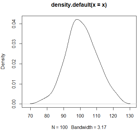
Density Plot: plot(density())
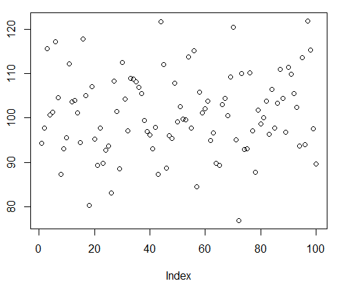
Scatter Plot: plot()
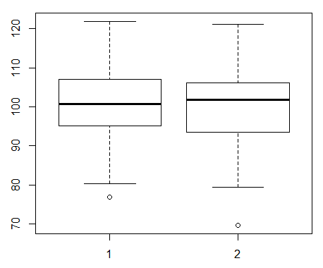
Box Plot: boxplot(time sex)
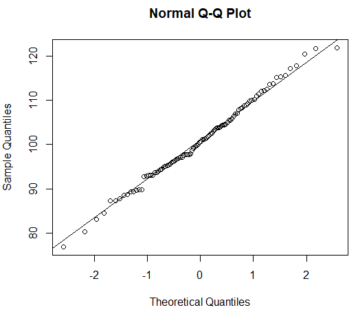
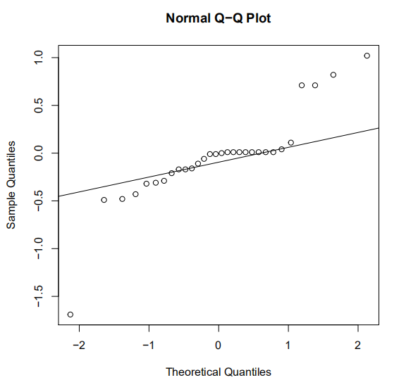
Q-Q Plot: qqnorm(), qqline() and qqplot()
#基本画图函数(直方图)
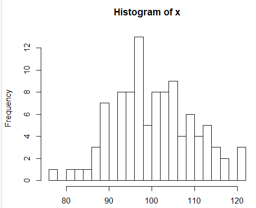
> set.seed(123)
> x=rnorm(100,mean=100,sd=10) #平均数100,方差10
> set.seed(234)
> y=rnorm(100,mean=100,sd=10)
> hist(x,breaks=20)
set.seed(123)
x=rnorm(100,mean=100,sd=10)
set.seed(234)
y=rnorm(100,mean=100,sd=10)
hist(x,breaks=20)
plot(density(x))
> set.seed(123)
> x=rnorm(100,mean=100,sd=10)
> set.seed(234)
> y=rnorm(100,mean=100,sd=10)
> hist(x,breaks=20)
> plot(density(x))
> plot(x)
> set.seed(123)
> x=rnorm(100,mean=100,sd=10)
> set.seed(234)
> y=rnorm(100,mean=100,sd=10)
> hist(x,breaks=20)
> plot(density(x))
> plot(x)
> boxplot(x,y)
> set.seed(123)
> x=rnorm(100,mean=100,sd=10)
> set.seed(234)
> y=rnorm(100,mean=100,sd=10)
> hist(x,breaks=20)
> plot(density(x))
> plot(x)
> boxplot(x,y)
> qqnorm(x)

> set.seed(123)
> x=rnorm(100,mean=100,sd=10)
> set.seed(234)
> y=rnorm(100,mean=100,sd=10)
> hist(x,breaks=20)
> plot(density(x))
> plot(x)
> qqnorm(x)
> qqline(x)
Lecture 02
1. Understanding the Dataset
1.1 Vector (向量)
Vectors are one-dimensional arrays that can hold numeric data, character data, or logical data. The combine function c() is used to form the vector.
(向量是一维数组,可以包含数字、字符、逻辑语句,用 c() 组成的向量)
> a = c(1, 2, 5, 3, 6, -2, 4)
> b = c("one", "two", "three")
> c = c(TRUE, TRUE, TRUE, FALSE, TRUE, FALSE)
1.2 Matrix (矩阵)
Matrix is a two-dimensional array where each element has the same mode (numeric, character, or logical). Matrices are created with the matrix() function.
(矩阵是一个二维数组,存储数据类型跟向量一样,通过 matrix() 实现)
x = matrix(1:20, nrow=5, ncol=4, byrow=TRUE)    # 1到20,5行4列
> x
     [,1] [,2] [,3] [,4]
[1,]    1    2    3    4
[2,]    5    6    7    8
[3,]    9   10   11   12
[4,]   13   14   15   16
[5,]   17   18   19   20

> x[2,]      #返回x第2行数据
[1] 5 6 7 8

> x[,2]      #返回x第2列数据
[1]  2  6 10 14 18

> x[1,4]      #返回x第1行,第4列数据
[1] 4

> x[2,c(2,4)]      #返回第2行,第2和第6个数
[1] 6 8

> x[3:5, 2]      #返回第2列,第3到第5行数
[1] 10 14 18


> y = matrix(1:20, nrow=5, ncol=4, byrow=FALSE)
> y
     [,1] [,2] [,3] [,4]
[1,]    1    6   11   16
[2,]    2    7   12   17
[3,]    3    8   13   18
[4,]    4    9   14   19
[5,]    5   10   15   20


> rnames=c("apple","banana","orange","melon","corn")
> cnames=c("cat","dog","bird","pig")
> x = matrix(1:20, nrow=5, ncol=4, byrow=TRUE)
> rownames(x)=rnames
> colnames(x)=cnames
> x      #对x的行和列赋名
       cat dog bird pig
apple    1   2    3   4
banana   5   6    7   8
orange   9  10   11  12
melon   13  14   15  16
corn    17  18   19  20
1.3 Array (多维数组)
Arrays are similar to matrices but can have more than two dimensions.They are created with an array() function.
> dim1 = c("A1", "A2")
> dim2 = c("B1", "B2", "B3")
> dim3 = c("C1", "C2", "C3", "C4")
> dim4 = c("D1", "D2", "D3")
> z = array(1:72, c(2, 3, 4, 3), dimnames=list(dim1, dim2, dim3, dim4))
> z
, , C1, D1

   B1 B2 B3
A1  1  3  5
A2  2  4  6

, , C2, D1

   B1 B2 B3
A1  7  9 11
A2  8 10 12

, , C3, D1

   B1 B2 B3
A1 13 15 17
A2 14 16 18

, , C4, D1

   B1 B2 B3
A1 19 21 23
A2 20 22 24

, , C1, D2

   B1 B2 B3
A1 25 27 29
A2 26 28 30

, , C2, D2

   B1 B2 B3
A1 31 33 35
A2 32 34 36

, , C3, D2

   B1 B2 B3
A1 37 39 41
A2 38 40 42

, , C4, D2

   B1 B2 B3
A1 43 45 47
A2 44 46 48

, , C1, D3

   B1 B2 B3
A1 49 51 53
A2 50 52 54

, , C2, D3

   B1 B2 B3
A1 55 57 59
A2 56 58 60

, , C3, D3

   B1 B2 B3
A1 61 63 65
A2 62 64 66

, , C4, D3

   B1 B2 B3
A1 67 69 71
A2 68 70 72

> z[1,2,3,]      # A1,B2,C3
D1 D2 D3
15 39 63
1.4 Data Frame ()
A data frame is more general than a matrix in that different columns can contain different modes of data (numeric, character, etc.). It is similar to the datasets you would typically see in SAS, SPSS, and Stata. Data frames are the most common data structure you will deal with in R.
> patientID = c(1, 2, 3, 4)
> age = c(25, 34, 28, 52)
> diabetes = c("Type1", "Type2", "Type1", "Type1")
> status = c("Poor", "Improved", "Excellent", "Poor")
> patientdata = data.frame(patientID, age, diabetes, status)
> patientdata
  patientID age diabetes    status
1         1  25    Type1      Poor
2         2  34    Type2  Improved
3         3  28    Type1 Excellent
4         4  52    Type1      Poor

> swim = read.csv("http://www.macalester.edu/~kaplan/ISM/datasets/swim100m.csv")
> patientdata[1:2]      #取前2列的内容
  patientID age
1         1  25
2         2  34
3         3  28
4         4  52

> patientdata[1:3]      #取前3列的内容
  patientID age diabetes
1         1  25    Type1
2         2  34    Type2
3         3  28    Type1
4         4  52    Type1

> patientdata[1,1:3]      #取第1行的前3列的内容
  patientID age diabetes
1         1  25    Type1

> patientdata[c(1,3),1:3]      #取第1行到第3行前3列的内容
  patientID age diabetes
1         1  25    Type1
3         3  28    Type1

> patientdata[1:2,]
  patientID age diabetes   status
1         1  25    Type1     Poor
2         2  34    Type2 Improved
1.5 Attach and Detach
The attach() function adds the data frame to the R search path.
The detach() function removes the data frame from the search path.
> attach(mtcars)
> layout(matrix(c(1,1,2,3), 2, 2, byrow = TRUE))
> hist(wt)
> hist(mpg)
> hist(disp)
> detach(mtcars)

> mtcars
                     mpg cyl  disp  hp drat
Mazda RX4           21.0   6 160.0 110 3.90
Mazda RX4 Wag       21.0   6 160.0 110 3.90
Datsun 710          22.8   4 108.0  93 3.85
Hornet 4 Drive      21.4   6 258.0 110 3.08
Hornet Sportabout   18.7   8 360.0 175 3.15
Valiant             18.1   6 225.0 105 2.76
Duster 360          14.3   8 360.0 245 3.21
Merc 240D           24.4   4 146.7  62 3.69
Merc 230            22.8   4 140.8  95 3.92
Merc 280            19.2   6 167.6 123 3.92
Merc 280C           17.8   6 167.6 123 3.92
Merc 450SE          16.4   8 275.8 180 3.07
Merc 450SL          17.3   8 275.8 180 3.07
Merc 450SLC         15.2   8 275.8 180 3.07
Cadillac Fleetwood  10.4   8 472.0 205 2.93
Lincoln Continental 10.4   8 460.0 215 3.00
Chrysler Imperial   14.7   8 440.0 230 3.23
Fiat 128            32.4   4  78.7  66 4.08
Honda Civic         30.4   4  75.7  52 4.93
Toyota Corolla      33.9   4  71.1  65 4.22
Toyota Corona       21.5   4 120.1  97 3.70
Dodge Challenger    15.5   8 318.0 150 2.76
AMC Javelin         15.2   8 304.0 150 3.15
Camaro Z28          13.3   8 350.0 245 3.73
Pontiac Firebird    19.2   8 400.0 175 3.08
Fiat X1-9           27.3   4  79.0  66 4.08
Porsche 914-2       26.0   4 120.3  91 4.43
Lotus Europa        30.4   4  95.1 113 3.77
Ford Pantera L      15.8   8 351.0 264 4.22
Ferrari Dino        19.7   6 145.0 175 3.62
Maserati Bora       15.0   8 301.0 335 3.54
Volvo 142E          21.4   4 121.0 109 4.11
                       wt  qsec vs am gear
Mazda RX4           2.620 16.46  0  1    4
Mazda RX4 Wag       2.875 17.02  0  1    4
Datsun 710          2.320 18.61  1  1    4
Hornet 4 Drive      3.215 19.44  1  0    3
Hornet Sportabout   3.440 17.02  0  0    3
Valiant             3.460 20.22  1  0    3
Duster 360          3.570 15.84  0  0    3
Merc 240D           3.190 20.00  1  0    4
Merc 230            3.150 22.90  1  0    4
Merc 280            3.440 18.30  1  0    4
Merc 280C           3.440 18.90  1  0    4
Merc 450SE          4.070 17.40  0  0    3
Merc 450SL          3.730 17.60  0  0    3
Merc 450SLC         3.780 18.00  0  0    3
Cadillac Fleetwood  5.250 17.98  0  0    3
Lincoln Continental 5.424 17.82  0  0    3
Chrysler Imperial   5.345 17.42  0  0    3
Fiat 128            2.200 19.47  1  1    4
Honda Civic         1.615 18.52  1  1    4
Toyota Corolla      1.835 19.90  1  1    4
Toyota Corona       2.465 20.01  1  0    3
Dodge Challenger    3.520 16.87  0  0    3
AMC Javelin         3.435 17.30  0  0    3
Camaro Z28          3.840 15.41  0  0    3
Pontiac Firebird    3.845 17.05  0  0    3
Fiat X1-9           1.935 18.90  1  1    4
Porsche 914-2       2.140 16.70  0  1    5
Lotus Europa        1.513 16.90  1  1    5
Ford Pantera L      3.170 14.50  0  1    5
Ferrari Dino        2.770 15.50  0  1    5
Maserati Bora       3.570 14.60  0  1    5
Volvo 142E          2.780 18.60  1  1    4
                    carb
Mazda RX4              4
Mazda RX4 Wag          4
Datsun 710             1
Hornet 4 Drive         1
Hornet Sportabout      2
Valiant                1
Duster 360             4
Merc 240D              2
Merc 230               2
Merc 280               4
Merc 280C              4
Merc 450SE             3
Merc 450SL             3
Merc 450SLC            3
Cadillac Fleetwood     4
Lincoln Continental    4
Chrysler Imperial      4
Fiat 128               1
Honda Civic            2
Toyota Corolla         1
Toyota Corona          1
Dodge Challenger       2
AMC Javelin            2
Camaro Z28             4
Pontiac Firebird       2
Fiat X1-9              1
Porsche 914-2          2
Lotus Europa           2
Ford Pantera L         4
Ferrari Dino           6
Maserati Bora          8
Volvo 142E             2
> mpg
 [1] 21.0 21.0 22.8 21.4 18.7 18.1 14.3 24.4
 [9] 22.8 19.2 17.8 16.4 17.3 15.2 10.4 10.4
[17] 14.7 32.4 30.4 33.9 21.5 15.5 15.2 13.3
[25] 19.2 27.3 26.0 30.4 15.8 19.7 15.0 21.4
1.6 List
Lists are the most complex of the R data types. Basically, a list is an ordered
collection of objects (components). A list allows you to gather a variety of
(possibly unrelated) objects under one name.
> mylist = list(patientdata, swim, x)
> mylist
[[1]]
patientID age diabetes status
1 1 25 Type1 Poor
2 2 34 Type2 Improved
3 3 28 Type1 Excellent
4 4 52 Type1 Poor
[[2]]
year time sex
1 1905 65.80 M
2 1908 65.60 M
3 1910 62.80 M
4 1912 61.60 M
5 1918 61.40 M
6 1920 60.40 M
7 1922 58.60 M
8 1924 57.40 M
9 1934 56.80 M
10 1935 56.60 M
11 1936 56.40 M
12 1944 55.90 M
13 1947 55.80 M
14 1948 55.40 M
15 1955 54.80 M
16 1957 54.60 M
17 1961 53.60 M
18 1964 52.90 M
19 1967 52.60 M
20 1968 52.20 M
21 1970 51.90 M
22 1972 51.22 M
23 1975 50.59 M
24 1976 49.44 M
25 1981 49.36 M
26 1985 49.24 M
27 1986 48.74 M
28 1988 48.42 M
29 1994 48.21 M
30 2000 48.18 M
31 2000 47.84 M
32 1908 95.00 F
33 1910 86.60 F
34 1911 84.60 F
35 1912 78.80 F
36 1915 76.20 F
37 1920 73.60 F
38 1923 72.80 F
39 1924 72.20 F
40 1926 70.00 F
41 1929 69.40 F
42 1930 68.00 F
43 1931 66.60 F
44 1933 66.00 F
45 1934 65.40 F
46 1936 64.60 F
47 1956 62.00 F
48 1958 61.20 F
49 1960 60.20 F
50 1962 59.50 F
51 1964 58.90 F
52 1972 58.50 F
53 1973 57.54 F
54 1974 56.96 F
55 1976 55.65 F
56 1978 55.41 F
57 1980 54.79 F
58 1986 54.73 F
59 1992 54.48 F
60 1994 54.01 F
61 2000 53.77 F
62 2004 53.52 F
[[3]]
cat dog bird pig
apple 1 2 3 4
banana 5 6 7 8
orange 9 10 11 12
melon 13 14 15 16
corn 17 18 19 20
2. Graphs
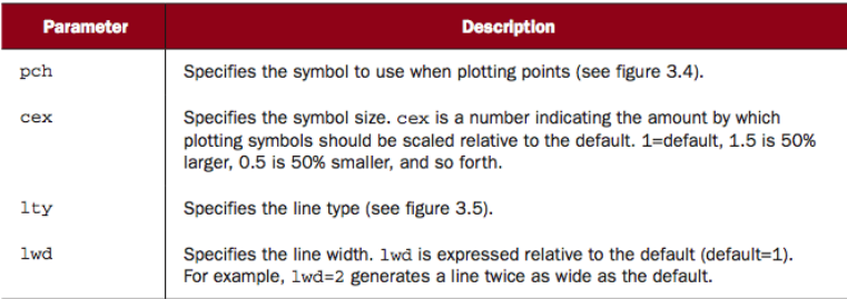
2.1 Graphical parameters
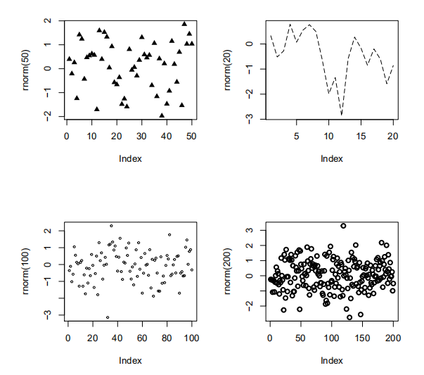
You can customize many features of a graph (fonts, colors, axes, titles) through options called graphical parameters. They are specified with an par() function.
> par(mfrow=c(2,2))
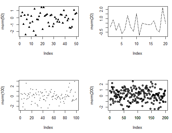
> plot(rnorm(50),pch=17) # pch=17,50个随机数,平均数是0
> plot(rnorm(20),type="l",lty=5) # lty=5,20个数,line→line type
> plot(rnorm(100),cex=0.5) # cex=0.5,100个正态分布随机数,大小为原来的0.5
> plot(rnorm(200),lwd=2) # lwd=2,200个随机数,粗细为原来的2倍

2.2 Text, Axes, and Legends
title()
axis()
legend()
> axis(1)
2.3 Layout
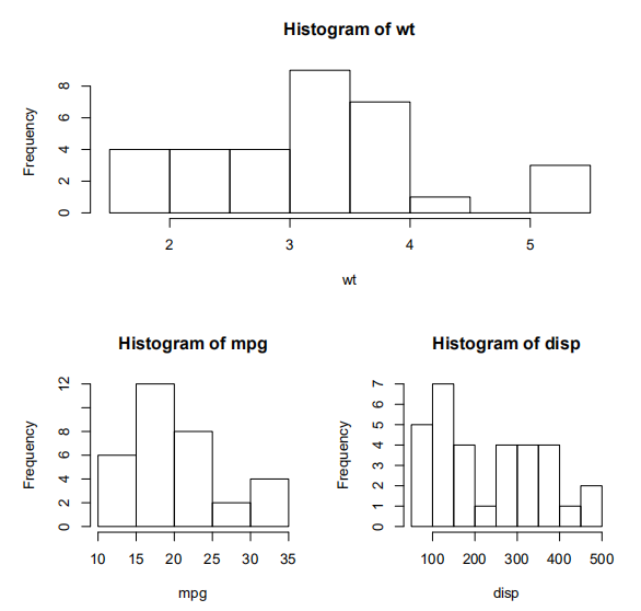
The layout() function has the form layout(mat) where mat is a matrix object speci- fying the location of the multiple plots to combine.
> attach(mtcars)
The following objects are masked from mtcars (pos = 3):

    am, carb, cyl, disp, drat, gear, hp,
    mpg, qsec, vs, wt

> layout(matrix(c(1,1,2,3), 2, 2, byrow = TRUE))
# layout() 输入一个矩阵,2行2列,
#第1个图占两个1,第2个图占2,第3个图占3
> hist(wt)
> hist(mpg)
> hist(disp)
> detach(mtcars)
> mylist[1]
[[1]]
   year  time sex
1  1905 65.80   M
2  1908 65.60   M
3  1910 62.80   M
4  1912 61.60   M
5  1918 61.40   M
6  1920 60.40   M
7  1922 58.60   M
8  1924 57.40   M
9  1934 56.80   M
10 1935 56.60   M
11 1936 56.40   M
12 1944 55.90   M
13 1947 55.80   M
14 1948 55.40   M
15 1955 54.80   M
16 1957 54.60   M
17 1961 53.60   M
18 1964 52.90   M
19 1967 52.60   M
20 1968 52.20   M
21 1970 51.90   M
22 1972 51.22   M
23 1975 50.59   M
24 1976 49.44   M
25 1981 49.36   M
26 1985 49.24   M
27 1986 48.74   M
28 1988 48.42   M
29 1994 48.21   M
30 2000 48.18   M
31 2000 47.84   M
32 1908 95.00   F
33 1910 86.60   F
34 1911 84.60   F
35 1912 78.80   F
36 1915 76.20   F
37 1920 73.60   F
38 1923 72.80   F
39 1924 72.20   F
40 1926 70.00   F
41 1929 69.40   F
42 1930 68.00   F
43 1931 66.60   F
44 1933 66.00   F
45 1934 65.40   F
46 1936 64.60   F
47 1956 62.00   F
48 1958 61.20   F
49 1960 60.20   F
50 1962 59.50   F
51 1964 58.90   F
52 1972 58.50   F
53 1973 57.54   F
54 1974 56.96   F
55 1976 55.65   F
56 1978 55.41   F
57 1980 54.79   F
58 1986 54.73   F
59 1992 54.48   F
60 1994 54.01   F
61 2000 53.77   F
62 2004 53.52   F
3. Next Topic
Operators, Control Flow & User-defined Function
Lecture 03
1. Last Lecture - List
> x = matrix(1:20, nrow=5, ncol=4, byrow=TRUE)
> swim = read.csv("http://www.macalester.edu/~kaplan/ISM/datasets/swim100m.csv")
> mylist=list(swim,x)    # 创建mylist,包含swim和x

> mylist[2]
[[1]]
     [,1] [,2] [,3] [,4]
[1,]    1    2    3    4
[2,]    5    6    7    8
[3,]    9   10   11   12
[4,]   13   14   15   16
[5,]   17   18   19   20

> mylist[[2]][2]    #返回mylist第2部分的第2个元素(默认竖向)
[1] 5
> mylist[[2]][3]
[1] 9

> mylist[[2]][1:2]    #返回mylist第2部分的前2个元素
[1] 1 5
> mylist[[2]][1:2,3]    #1,2两行,第3列
[1] 3 7
> mylist[[2]][1:2,]    #1,2两行
     [,1] [,2] [,3] [,4]
[1,]    1    2    3    4
[2,]    5    6    7    8
2. Operators
( “three value logic”-三值逻辑 )
>, >=, <, <=, ==, !=(不等于), x | y(或), x & y(且)
3. Control Flow
3.1 Repetition and looping
Looping constructs repetitively execute a statement or series of statements until a condition is not true. These include the for and while structures.
> #For-Loop
> for(i in 1:10){      # 1到10
+   print(i)
+ }
[1] 1
[1] 2
[1] 3
[1] 4
[1] 5
[1] 6
[1] 7
[1] 8
[1] 9
[1] 10

> #While-Loop
> i = 1
> while(i <= 10){      # 1到10
+   print(i)
+   i=i+1
+ }
[1] 1
[1] 2
[1] 3
[1] 4
[1] 5
[1] 6
[1] 7
[1] 8
[1] 9
[1] 10
3.2 Conditional Execution
In conditional execution, a statement or statements are only executed if a specified condition is met. These constructs include if, if-else, and switch.
> #If statement
> i = 1
> if(i == 1){
+   print("Hello World")
+ }
[1] "Hello World"

> #If-else statement
> i = 2
> if(i == 1){
+   print("Hello World!")
+ }else{
+   print("Goodbye World!")
+ }
[1] "Goodbye World!"

> #switch
> #switch(expression, cnoditions)
> feelings = c("sad", "afraid")
> for (i in feelings){
+   print(
+     switch(i,
+            happy  = "I am glad you are happy",
+            afraid = "There is nothing to fear",
+            sad    = "Cheer up",
+            angry  = "Calm down now"
+     )
+   )
+ }
[1] "Cheer up"
[1] "There is nothing to fear"
4. User-defined Function
One of greatest strengths of R is the ability to add functions. In fact, many of the functions in R are functions of existing functions.
> myfunction = function(x,a,b,c){
+ return(a*sin(x)^2 - b*x + c)
+ }
> curve(myfunction(x,20,3,4),xlim=c(1,20))

> curve(exp(x),xlim=c(1,20))

> myfeeling = function(x){
+   for (i in x){
+     print(
+       switch(i,
+              happy  = "I am glad you are happy",
+              afraid = "There is nothing to fear",
+              sad    = "Cheer up",
+              angry  = "Calm down now"
+       )
+     )
+   }
+ }
> feelings = c("sad", "afraid")
> myfeeling(feelings)
[1] "Cheer up"
[1] "There is nothing to fear"
Lecture 04
1. Baisc Graph
1.1 Bar Plot (柱状图)
>library(vcd)
>counts = table(Arthritis$Improved)
>counts
None Some Marked
42 14 28

> par(mfrow=c(2,2))      # 创建2×2网格
> barplot(counts,
+         main="Simple Bar Plot",
+         xlab="Improvement", ylab="Frequency")

> barplot(counts,
+         main="Horizontal Bar Plot",
+         xlab="Frequency", ylab="Improvement",
+         horiz=TRUE)

> counts <- table(Arthritis$Improved, Arthritis$Treatment)
> counts
Placebo Treated
None 29 13
Some 7 7
Marked 7 21

> barplot(counts,
+         main="Stacked Bar Plot",
+         xlab="Treatment", ylab="Frequency",
+         col=c("red", "yellow","green"),
+         legend=rownames(counts))

> barplot(counts,
+         main="Grouped Bar Plot",
+         xlab="Treatment", ylab="Frequency",
+         col=c("red", "yellow", "green"),
+         legend=rownames(counts), beside=TRUE)
>

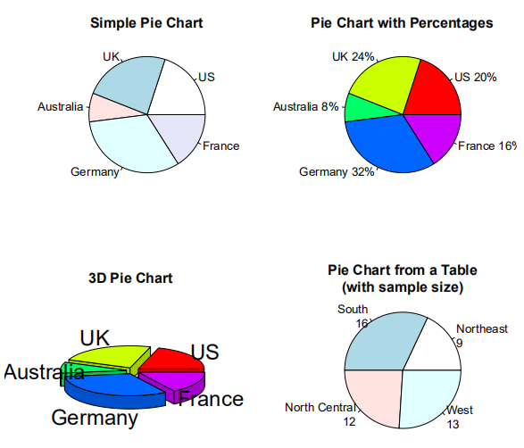
1.2 Pie Chart (饼图)
> library(plotrix)

#饼图
> par(mfrow=c(2,2))
> slices <- c(10, 12,4, 16, 8)      #数据来源
> lbls <- c("US", "UK", "Australia", "Germany", "France")
> pie(slices, labels = lbls,main="Simple Pie Chart",edges=300,radius=1)      #edges方格大小,radius圆的半径
> lbls2      #查看比例,百分数
[1] "US 20%"       "UK 24%"       "Australia 8%"
[4] "Germany 32%"  "France 16%"

#百分数饼图
> pct <- round(slices/sum(slices)*100)
> lbls2 <- paste(lbls, " ", pct, "%", sep="")
> pie(slices, labels=lbls2, col=rainbow(length(lbls2)),
+     main="Pie Chart with Percentages",edges=300,radius=1)

#3D图
> pie3D(slices, labels=lbls,explode=0.5,      #explode图表分离程度:0贴合,0.1分开一点
+       main="3D Pie Chart ",edges=300,radius=1)

> mytable <- table(state.region)      #table(state.region)美国一些州的数据
> lbls3 <- paste(names(mytable), "\n", mytable, sep="")      #\n:new line

#
> pie(mytable,labels=lbls3,
+     main="Pie Chart from a Table\n(with sample size)",
+     edges=300,radius=1)
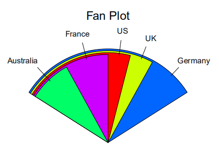
1.3 Fan Plot (扇形图)
#会自动填充颜色
> slices <- c(10, 12,4, 16, 8)
> lbls <- c("US", "UK", "Australia", "Germany", "France")
> fan.plot(slices, labels = lbls, main="Fan Plot")
1.4 Dot Plot (点图)
> dotchart(mtcars$mpg,       # 内置函数, mpg英里每加仑
+          labels=row.names(mtcars),cex=0.7,
+          main="Gas Mileage for Car Models",
+          xlab="Miles Per Gallon")

2. Basic Statistics
2.1 Descriptive statistics
> head(mtcars)
#展示数据框架的前几行
                   mpg cyl disp  hp drat    wt
Mazda RX4         21.0   6  160 110 3.90 2.620
Mazda RX4 Wag     21.0   6  160 110 3.90 2.875
Datsun 710        22.8   4  108  93 3.85 2.320
Hornet 4 Drive    21.4   6  258 110 3.08 3.215
Hornet Sportabout 18.7   8  360 175 3.15 3.440
Valiant           18.1   6  225 105 2.76 3.460
                   qsec vs am gear carb
Mazda RX4         16.46  0  1    4    4
Mazda RX4 Wag     17.02  0  1    4    4
Datsun 710        18.61  1  1    4    1
Hornet 4 Drive    19.44  1  0    3    1
Hornet Sportabout 17.02  0  0    3    2
Valiant           20.22  1  0    3    1

> summary(mtcars)
#展示重要数据的特征,数据基本结构
#自动了11个变量(mtcars内置11个变量)
      mpg             cyl             disp
 Min.   :10.40   Min.   :4.000   Min.   : 71.1
 1st Qu.:15.43   1st Qu.:4.000   1st Qu.:120.8
 Median :19.20   Median :6.000   Median :196.3
 Mean   :20.09   Mean   :6.188   Mean   :230.7
 3rd Qu.:22.80   3rd Qu.:8.000   3rd Qu.:326.0
 Max.   :33.90   Max.   :8.000   Max.   :472.0
       hp             drat             wt
 Min.   : 52.0   Min.   :2.760   Min.   :1.513
 1st Qu.: 96.5   1st Qu.:3.080   1st Qu.:2.581
 Median :123.0   Median :3.695   Median :3.325
 Mean   :146.7   Mean   :3.597   Mean   :3.217
 3rd Qu.:180.0   3rd Qu.:3.920   3rd Qu.:3.610
 Max.   :335.0   Max.   :4.930   Max.   :5.424
      qsec             vs
 Min.   :14.50   Min.   :0.0000
 1st Qu.:16.89   1st Qu.:0.0000
 Median :17.71   Median :0.0000
 Mean   :17.85   Mean   :0.4375
 3rd Qu.:18.90   3rd Qu.:1.0000
 Max.   :22.90   Max.   :1.0000
       am              gear
 Min.   :0.0000   Min.   :3.000
 1st Qu.:0.0000   1st Qu.:3.000
 Median :0.0000   Median :4.000
 Mean   :0.4062   Mean   :3.688
 3rd Qu.:1.0000   3rd Qu.:4.000
 Max.   :1.0000   Max.   :5.000
      carb
 Min.   :1.000
 1st Qu.:2.000
 Median :2.000
 Mean   :2.812
 3rd Qu.:4.000
 Max.   :8.000
2.2 Frequency and contingency tables
#Tables
> attach(mtcars)      #将列的名字直接当做变量名来用
The following objects are masked from mtcars (pos = 3):

    am, carb, cyl, disp, drat, gear, hp,
    mpg, qsec, vs, wt

> table(cyl)
 #气缸:32个样本,4气缸的11个,6气缸的7个,8气缸的14个
#用cut()确定范围
cyl
 4  6  8
11  7 14
> summary(mpg)      #油耗
   Min. 1st Qu.  Median    Mean 3rd Qu.    Max.
  10.40   15.43   19.20   20.09   22.80   33.90
> table(cut(mpg,seq(10,34,by=2)))
# seq():生成10到34,每2个递增的数计算范围

(10,12] (12,14] (14,16] (16,18] (18,20] (20,22]
      2       1       7       3       5       5
(22,24] (24,26] (26,28] (28,30] (30,32] (32,34]
      2       2       1       0       2       2
2.3 Correlations
> states = state.x77[,1:6]
> cov(states)      #协方差
              Population      Income
Population 19931683.7588 571229.7796
Income       571229.7796 377573.3061
Illiteracy      292.8680   -163.7020
Life Exp       -407.8425    280.6632
Murder         5663.5237   -521.8943
HS Grad       -3551.5096   3076.7690
             Illiteracy     Life Exp      Murder
Population  292.8679592 -407.8424612 5663.523714
Income     -163.7020408  280.6631837 -521.894286
Illiteracy    0.3715306   -0.4815122    1.581776
Life Exp     -0.4815122    1.8020204   -3.869480
Murder        1.5817755   -3.8694804   13.627465
HS Grad      -3.2354694    6.3126849  -14.549616
                HS Grad
Population -3551.509551
Income      3076.768980
Illiteracy    -3.235469
Life Exp       6.312685
Murder       -14.549616
HS Grad       65.237894
> var(states)
              Population      Income
Population 19931683.7588 571229.7796
Income       571229.7796 377573.3061
Illiteracy      292.8680   -163.7020
Life Exp       -407.8425    280.6632
Murder         5663.5237   -521.8943
HS Grad       -3551.5096   3076.7690
             Illiteracy     Life Exp      Murder
Population  292.8679592 -407.8424612 5663.523714
Income     -163.7020408  280.6631837 -521.894286
Illiteracy    0.3715306   -0.4815122    1.581776
Life Exp     -0.4815122    1.8020204   -3.869480
Murder        1.5817755   -3.8694804   13.627465
HS Grad      -3.2354694    6.3126849  -14.549616
                HS Grad
Population -3551.509551
Income      3076.768980
Illiteracy    -3.235469
Life Exp       6.312685
Murder       -14.549616
HS Grad       65.237894

> cor(states)      #自动识别多列变量,两两对应分析
            Population     Income Illiteracy
Population  1.00000000  0.2082276  0.1076224
Income      0.20822756  1.0000000 -0.4370752
Illiteracy  0.10762237 -0.4370752  1.0000000
Life Exp   -0.06805195  0.3402553 -0.5884779
Murder      0.34364275 -0.2300776  0.7029752
HS Grad    -0.09848975  0.6199323 -0.6571886
              Life Exp     Murder     HS Grad
Population -0.06805195  0.3436428 -0.09848975
Income      0.34025534 -0.2300776  0.61993232
Illiteracy -0.58847793  0.7029752 -0.65718861
Life Exp    1.00000000 -0.7808458  0.58221620
Murder     -0.78084575  1.0000000 -0.48797102
HS Grad     0.58221620 -0.4879710  1.00000000
2.4 T-test (T检验)
> x = rnorm(100, mean = 10, sd = 1)
> y = rnorm(100, mean = 30, sd = 10)
#正态分布中的100个数,平均数分别是10和30,标准差是1和10
> t.test(x, y, alt = "two.sided",paired=TRUE)

	Paired t-test

data:  x and y
t = -21.481, df = 99, p-value < 2.2e-16
alternative hypothesis: true difference in means is not equal to 0
95 percent confidence interval:
 -21.51457 -17.87599
sample estimates:
mean of the differences
              -19.69528
> ?T-test
> ?wilcox.test
2.5 Nonparametric tests of group differences
> wilcox.test(x,y,alt="less")

	Wilcoxon rank sum test with continuity
	correction

data:  x and y
W = 130, p-value < 2.2e-16
alternative hypothesis: true location shift is less than 0
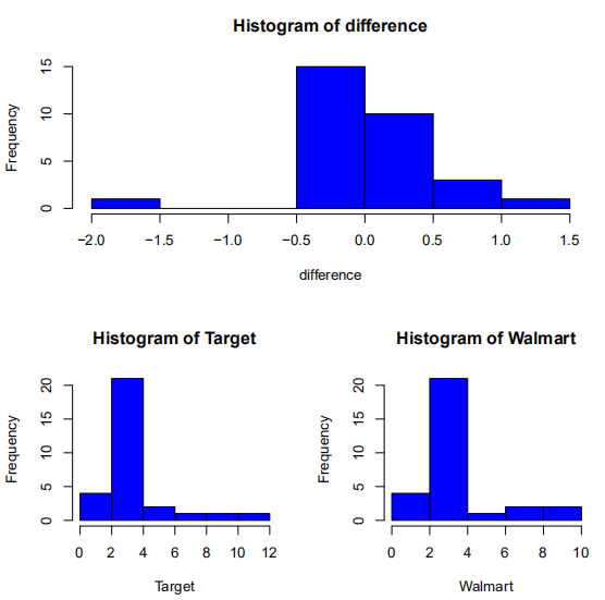
3. Practical Example
> data=read.csv("~/documents/R Programming/project/STAT.csv")
> attach(data)
> layout(matrix(c(1,1,2,3),2,2,byrow=TRUE))      #画3个条形图
> hist(difference,col="blue")
> hist(Target,col="blue")
> hist(Walmart,col="blue")
> par(mfrow=c(2,1))
> boxplot(data[2:4],horizontal=TRUE)
> boxplot(difference,horizontal=TRUE)
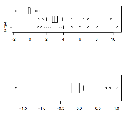
> par(mfrow=c(1,1))
> qqnorm(difference)
> qqline(difference)
> binom.test(length(difference[difference>=0]),
+            length(difference),
+            alter="two.sided")
Exact binomial test
data: length(difference[difference >= 0]) and length(difference)
number of successes = 15, number of trials = 30, p-value = 1
alternative hypothesis: true probability of success is not equal to 0.5
95 percent confidence interval:
0.3129703 0.6870297
sample estimates:
probability of success
0.5

> wilcox.test(difference,alter="two.sided")
Wilcoxon signed rank test with continuity correction
data: difference
V = 174.5, p-value = 0.3557
alternative hypothesis: true location is not equal to 0

> t.test(difference,alter="two.sided")
One Sample t-test
data: difference
t = -0.5432, df = 29, p-value = 0.5911
alternative hypothesis: true mean is not equal to 0
95 percent confidence interval:
-0.2255485 0.1308819
sample estimates:
mean of x
-0.04733333
> library(nortest)      #验证是不是正态分布的package
> ad.test(difference)
Anderson-Darling normality test
data: difference
A = 2.1234, p-value = 1.552e-05
Lecture 05
1. Matrix Algebra
R for MATLAB users: http://mathesaurus.sourceforge.net/octave-r.html(区分R和MATLAB的指令/外网)
> set.seed(123)      #100个数里随机取15个,5行3列
> A = matrix(sample(100,15), nrow=5, ncol=3)
> set.seed(234)
> B = matrix(sample(100,15), nrow=5, ncol=3)
> set.seed(321)
> X = matrix(sample(100,25), nrow=5, ncol=5)
> set.seed(213)
> b = matrix(sample(100,5),nrow=5, ncol=1)
> A
     [,1] [,2] [,3]
[1,]   31   42   90
[2,]   79   50   69
[3,]   51   43   57
[4,]   14   97    9
[5,]   67   25   72
> B
     [,1] [,2] [,3]
[1,]   97   18   55
[2,]   31   56   54
[3,]   34    1   63
[4,]   46   68   79
[5,]   98   92   43
> X
     [,1] [,2] [,3] [,4] [,5]
[1,]   54   17   82   36   51
[2,]   77   47   79   78   13
[3,]   88   11   75   34   30
[4,]   80   25   91    4   89
[5,]   58   31   90   48   81
> b
     [,1]
[1,]   56
[2,]   44
[3,]   16
[4,]   73
[5,]   61

#  + - * / ^
#Element-wise addition, subtraction, multiplication, division
#, and exponentiation, respectively.

> A + 2
     [,1] [,2] [,3]
[1,]   33   44   92
[2,]   81   52   71
[3,]   53   45   59
[4,]   16   99   11
[5,]   69   27   74
> A * 2
     [,1] [,2] [,3]
[1,]   62   84  180
[2,]  158  100  138
[3,]  102   86  114
[4,]   28  194   18
[5,]  134   50  144
> A ^ 2
     [,1] [,2] [,3]
[1,]  961 1764 8100
[2,] 6241 2500 4761
[3,] 2601 1849 3249
[4,]  196 9409   81
[5,] 4489  625 5184

#Matrix multiplication
> t(A) %*% B      # t(A): transports(A的转置矩阵)
      [,1]  [,2]  [,3]
[1,] 14400 12149 13171
[2,] 13998 12495 16457
[3,] 20277 12777 16074

#Returns a vector containing the column means of A.
> colMeans(A)
[1] 48.4 51.4 59.4

#Returns a vector containing the column sums of A.
> colSums(A)
[1] 242 257 297

> #Returns a vector containing the row means of A.
> rowMeans(A)      #每一行的平均数
[1] 54.33333 66.00000 50.33333 40.00000
[5] 54.66667

> #Returns a vector containing the row sums of A.
> rowSums(A)      #每一行的和
[1] 163 198 151 120 164

> #Matrix Crossproduct
> # A'A      # A×t(A)
> crossprod(A)      # 矩阵的叉乘
      [,1]  [,2]  [,3]
[1,] 14488 10478 16098
[2,] 10478 16147 12354
[3,] 16098 12354 21375

> # A'B
> crossprod(A,B)
      [,1]  [,2]  [,3]
[1,] 14400 12149 13171
[2,] 13998 12495 16457
[3,] 20277 12777 16074

> #Inverse of A where A is a square matrix.
> solve(X)      #
             [,1]         [,2]        [,3]         [,4]        [,5]
[1,] -0.038716716 -0.001615536  0.02639602  0.001865776  0.01281012
[2,] -0.007833594  0.029329714 -0.03505452  0.029705074 -0.01943073
[3,]  0.070634812  0.005604153 -0.02616163  0.007748418 -0.04419740
[4,] -0.022901322 -0.006899276  0.01956364 -0.026670636  0.03758562
[5,] -0.034190849 -0.012206525  0.01199028 -0.005509128  0.03744472

> #Solves for vector x in the equation b = Ax.
> # b = Xv
> v = solve(X, b)
> v
           [,1]
[1,] -0.8992643
[2,]  1.2741498
[3,]  1.6531390
[4,] -0.9272574
[5,] -0.3779688

> #Returns a vector containing the elements of the principal diagonal
> diag(X)      # 返回矩阵的对角线
[1] 54 47 75  4 81

> X
     [,1] [,2] [,3] [,4] [,5]
[1,]   54   17   82   36   51
[2,]   77   47   79   78   13
[3,]   88   11   75   34   30
[4,]   80   25   91    4   89
[5,]   58   31   90   48   81

> #Creates a diagonal matrix with the elements of x in the principal diagonal.
> diag(c(1,2,3,4))      # 创建对角线矩阵
     [,1] [,2] [,3] [,4]
[1,]    1    0    0    0
[2,]    0    2    0    0
[3,]    0    0    3    0
[4,]    0    0    0    4

> #If k is a scalar, this creates a k x k identity matrix.
> diag(5)      # diag(x): x行,x列的单位矩阵
     [,1] [,2] [,3] [,4] [,5]
[1,]    1    0    0    0    0
[2,]    0    1    0    0    0
[3,]    0    0    1    0    0
[4,]    0    0    0    1    0
[5,]    0    0    0    0    1

> #Eigenvalues and eigenvectors of A.
> eigen(X)      #本征函数
eigen() decomposition
$values
[1] 264.12614+ 0.00000i
[2] -39.97988+ 0.00000i
[3]  26.02694+12.60671i
[4]  26.02694-12.60671i
[5] -15.20015+ 0.00000i

$vectors
             [,1]           [,2]
[1,] 0.3893077+0i  0.08721116+0i
[2,] 0.4742054+0i  0.55199369+0i
[3,] 0.3745159+0i  0.10652480+0i
[4,] 0.4712054+0i -0.82000026+0i
[5,] 0.5111477+0i  0.06284292+0i
                        [,3]
[1,] -0.05950991+0.03631631i
[2,]  0.72745041+0.00000000i
[3,] -0.03767373+0.38696839i
[4,] -0.08196570-0.22750249i
[5,] -0.10038826-0.49622393i
                        [,4]
[1,] -0.05950991-0.03631631i
[2,]  0.72745041+0.00000000i
[3,] -0.03767373-0.38696839i
[4,] -0.08196570+0.22750249i
[5,] -0.10038826+0.49622393i
              [,5]
[1,] -0.5138367+0i
[2,]  0.2763409+0i
[3,]  0.6846989+0i
[4,] -0.3671550+0i
[5,] -0.2366265+0i

# or
> eigen(X)
eigen() decomposition
$values
[1] 264.12614+ 0.00000i -39.97988+ 0.00000i  26.02694+12.60671i  26.02694-12.60671i -15.20015+ 0.00000i

$vectors
             [,1]           [,2]                    [,3]                    [,4]          [,5]
[1,] 0.3893077+0i  0.08721116+0i -0.05950991+0.03631631i -0.05950991-0.03631631i -0.5138367+0i
[2,] 0.4742054+0i  0.55199369+0i  0.72745041+0.00000000i  0.72745041+0.00000000i  0.2763409+0i
[3,] 0.3745159+0i  0.10652480+0i -0.03767373+0.38696839i -0.03767373-0.38696839i  0.6846989+0i
[4,] 0.4712054+0i -0.82000026+0i -0.08196570-0.22750249i -0.08196570+0.22750249i -0.3671550+0i
[5,] 0.5111477+0i  0.06284292+0i -0.10038826-0.49622393i -0.10038826+0.49622393i -0.2366265+0i
2. Afterword
Google & English
The R Project (http://www.r-project.org/): The official R website and your first stop for all things R. The site includes extensive documentation, including An Introduction to R, The R Language Definition, Writing R Extensions, R Data Import/Export, R Installation and Administration, and The R FAQ.
(官方R网站)
The R Journal (http://journal.r-project.org/): A freely accessible refereed journal containing articles on the R project and contributed packages.
(R免费期刊)
R Bloggers (http://www.r-bloggers.com/): A central hub (blog aggregator) collecting content from bloggers writing about R. Contains new articles daily. I am addicted to it.
(R最新资讯,教程)
Planet R (http://planetr.stderr.org): Another good site-aggregator, including information from a wide range of sources. Updated daily.
R Graph Gallery (http://addictedtor.free.fr/graphiques/): A collection of
innovative graphs, along with their source code.
R Graphics Manual (http://bm2.genes.nig.ac.jp/): A collection of R graphics from all R packages, arranged by topic, package, and function. At last count, there were 35,000+ images!
(R作图技巧,提供源代码,包)
Journal of Statistical Software (http://www.jstatsoft.org/): A freely accessible refereed journal containing articles, book reviews, and code snippets on statistical computing. Contains frequent articles about R.
(学界统计学)
Quick-R (http://www.statmethods.net): The website of R in Action author.
(R author)
Lecture 06
Factors
> # FACTOR
> factor = factor(rep(c(1:3),times=5))
> factor
 [1] 1 2 3 1 2 3 1 2 3 1 2 3 1 2 3
Levels: 1 2 3

> X = sample(100,15)
> tapply(X,factor,mean)
   1    2    3
67.6 52.2 56.8

> rbind(X,factor)      # X用factor来标记
       [,1] [,2] [,3] [,4] [,5] [,6] [,7] [,8]
X        97   87   93   34   16   67   48   43
factor    1    2    3    1    2    3    1    2
       [,9] [,10] [,11] [,12] [,13] [,14] [,15]
X        25    77    21    60    82    94    39
factor    3     1     2     3     1     2     3

> boo = rbind(X,factor)[2,]==1      # 判断语句
> rbind(X,factor)[2,]==1
 [1]  TRUE FALSE FALSE  TRUE FALSE FALSE  TRUE
 [8] FALSE FALSE  TRUE FALSE FALSE  TRUE FALSE
[15] FALSE> rbind(X,factor)[2,]==1
 [1]  TRUE FALSE FALSE  TRUE FALSE FALSE  TRUE
 [8] FALSE FALSE  TRUE FALSE FALSE  TRUE FALSE
[15] FALSE

> which(boo)      # Ture
[1]  1  4  7 10 13

> rbind(X,factor)[1,which(boo)]
[1] 97 34 48 77 82

> sum(rbind(X,factor)[1,which(boo)])/length(which(boo))
[1] 67.6


 476
476


 被折叠的 条评论
为什么被折叠?
被折叠的 条评论
为什么被折叠?
 到【灌水乐园】发言


