 用PyTorch复现ViT论文并应用于图像分类


文章目录
机器学习研究论文的内容可能因论文而异,但通常遵循以下结构:
| Section | Contents |
|---|---|
| Abstract | 论文主要发现(贡献)的概述(总结)。 |
| Introduction | 本文的主要问题是什么以及之前用于尝试解决该问题的方法的详细信息。 |
| Method | 研究人员是如何进行研究的?例如,使用了什么模型、数据源、训练设置? |
| Results | 论文的结果是什么?如果使用新型模型或训练设置,研究结果与以前的工作相比如何? (这就是实验跟踪派上用场的地方) |
| Conclusion | 建议的方法有哪些局限性?研究界的下一步行动是什么? |
| References | 研究人员查看了哪些资源/其他论文来构建自己的工作体系? |
| Appendix | 是否有任何未包含在上述任何部分中的额外资源/发现可供查看? |
有几个地方可以找到和阅读机器学习研究论文(和代码):
| Resource | What is it? |
|---|---|
| arXiv | arXiv 发音为“archive”,是一个免费开放的资源,用于阅读从物理到计算机科学(包括机器学习)等各个领域的技术文章。 |
| AK Twitter | AK Twitter 帐户发布机器学习研究亮点,几乎每天都会进行现场演示。 |
| Papers with Code | 精选的热门、活跃和最优秀的机器学习论文集,其中许多包含附加的代码资源。还包括一系列常见的机器学习数据集、基准测试和当前最先进的模型。 |
| lucidrains’ vit-pytorch GitHub repository | vit-pytorch 存储库是使用 PyTorch 代码 复现的各种研究论文中的 Vision Transformer 模型架构的集合。 |
本篇内容:
使用 PyTorch 复现机器学习研究论文 An Image is Worth 16x16 Words: Transformers for Image Recognition at Scale(ViT paper)。
Transformer 架构通常被认为是任何使用注意力机制作为其主要学习层的神经网络。类似于卷积神经网络 (CNN) 如何使用卷积作为其主要学习层。
Vision Transformer (ViT) 架构旨在使原始 Transformer 架构适应视觉问题(分类是第一个,之后还有许多其他分类)。
最初的 Vision Transformer 在过去几年中经历了多次迭代,但是,本文将专注于根据原始 ViT 论文构建 ViT 架构并将其应用于 FoodVision Mini。
关于FoodVision Mini数据集可查看前面博客。
本文主要包含以下内容:
- 进行设置:引入基础库,以及引入前面章节可以重复使用的函数。
- 获取数据:和前面博客保持一致,使用的披萨、牛排和寿司图像分类数据集,并构建一个 Vision Transformer 来尝试改进 FoodVision Mini 模型的结果。
- 创建Dataset和DataLoader:重复使用
data_setup.py脚本来设置我们的 DataLoaders。 - 复现ViT论文
- Equation 1: The Patch Embedding:ViT 架构由四个主要公式组成,第一个是 patch 和位置嵌入。或者将图像转换为一系列可学习的 patch 。
- Equation 2: Multi-Head Attention (MSA)【多头注意力】:自注意力/多头自注意力(MSA)机制是每个 Transformer 架构(包括 ViT 架构)的核心,使用 PyTorch 的内置层创建一个 MSA 块。
- Equation 3: Multilayer Perceptron (MLP)【多层感知机】:ViT 架构使用多层感知器作为其 Transformer Encoder 的一部分及其输出层。首先为 Transformer Encoder 创建 MLP。
- 创建 Transformer 编码器(encode):Transformer 编码器通常由通过残差连接连接在一起的 MSA(公式 2)和 MLP(公式 3)的交替层组成。
- 将它们放在一起创建 ViT
- 为 ViT 模型设置训练代码:可以重复使用前面博客的
engine.py中的train()函数 - 使用来自 torchvision.models 的预训练 ViT :训练像 ViT 这样的大型模型通常需要大量数据。由于我们只处理少量的披萨、牛排和寿司图像,看看是否可以利用迁移学习的力量来提高性能。
- 对自定义图像进行预测
0. 进行设置
补充需要使用到之前编写过的python脚本:【可以从前面博客找到】
data_setup.py : 创建DataLoader
"""
Contains functionality for creating PyTorch DataLoaders for
image classification data.
"""
import os

from torchvision import datasets, transforms
from torch.utils.data import DataLoader

NUM_WORKERS = os.cpu_count()


def create_dataloaders(
        train_dir: str,
        test_dir: str,
        transform: transforms.Compose,
        batch_size: int,
        num_workers: int = NUM_WORKERS
):
    """Creates training and testing DataLoaders.

  Takes in a training directory and testing directory path and turns
  them into PyTorch Datasets and then into PyTorch DataLoaders.

  Args:
    train_dir: Path to training directory.
    test_dir: Path to testing directory.
    transform: torchvision transforms to perform on training and testing data.
    batch_size: Number of samples per batch in each of the DataLoaders.
    num_workers: An integer for number of workers per DataLoader.

  Returns:
    A tuple of (train_dataloader, test_dataloader, class_names).
    Where class_names is a list of the target classes.
    Example usage:
      train_dataloader, test_dataloader, class_names = \
        = create_dataloaders(train_dir=path/to/train_dir,
                             test_dir=path/to/test_dir,
                             transform=some_transform,
                             batch_size=32,
                             num_workers=4)
  """
    # Use ImageFolder to create dataset(s)
    train_data = datasets.ImageFolder(train_dir, transform=transform)
    test_data = datasets.ImageFolder(test_dir, transform=transform)

    # Get class names
    class_names = train_data.classes

    # Turn images into data loaders
    train_dataloader = DataLoader(
        train_data,
        batch_size=batch_size,
        shuffle=True,
        num_workers=num_workers,
        pin_memory=True,
    )
    test_dataloader = DataLoader(
        test_data,
        batch_size=batch_size,
        shuffle=False,
        num_workers=num_workers,
        pin_memory=True,
    )

    return train_dataloader, test_dataloader, class_names
engine.py :包含各种训练函数
"""
Contains functions for training and testing a PyTorch model.
"""
import torch

from tqdm.auto import tqdm
from typing import Dict, List, Tuple


def train_step(model: torch.nn.Module,
               dataloader: torch.utils.data.DataLoader,
               loss_fn: torch.nn.Module,
               optimizer: torch.optim.Optimizer,
               device: torch.device) -> Tuple[float, float]:
    """Trains a PyTorch model for a single epoch.

    Turns a target PyTorch model to training mode and then
    runs through all of the required training steps (forward
    pass, loss calculation, optimizer step).

    Args:
    model: A PyTorch model to be trained.
    dataloader: A DataLoader instance for the model to be trained on.
    loss_fn: A PyTorch loss function to minimize.
    optimizer: A PyTorch optimizer to help minimize the loss function.
    device: A target device to compute on (e.g. "cuda" or "cpu").

    Returns:
    A tuple of training loss and training accuracy metrics.
    In the form (train_loss, train_accuracy). For example:

    (0.1112, 0.8743)
    """
    # Put model in train mode
    model.train()

    # Setup train loss and train accuracy values
    train_loss, train_acc = 0, 0

    # Loop through data loader data batches
    for batch, (X, y) in enumerate(dataloader):
        # Send data to target device
        X, y = X.to(device), y.to(device)

        # 1. Forward pass
        y_pred = model(X)

        # 2. Calculate  and accumulate loss
        loss = loss_fn(y_pred, y)
        train_loss += loss.item()

        # 3. Optimizer zero grad
        optimizer.zero_grad()

        # 4. Loss backward
        loss.backward()

        # 5. Optimizer step
        optimizer.step()

        # Calculate and accumulate accuracy metric across all batches
        y_pred_class = torch.argmax(torch.softmax(y_pred, dim=1), dim=1)
        train_acc += (y_pred_class == y).sum().item() / len(y_pred)

    # Adjust metrics to get average loss and accuracy per batch
    train_loss = train_loss / len(dataloader)
    train_acc = train_acc / len(dataloader)
    return train_loss, train_acc


def test_step(model: torch.nn.Module,
              dataloader: torch.utils.data.DataLoader,
              loss_fn: torch.nn.Module,
              device: torch.device) -> Tuple[float, float]:
    """Tests a PyTorch model for a single epoch.

    Turns a target PyTorch model to "eval" mode and then performs
    a forward pass on a testing dataset.

    Args:
    model: A PyTorch model to be tested.
    dataloader: A DataLoader instance for the model to be tested on.
    loss_fn: A PyTorch loss function to calculate loss on the test data.
    device: A target device to compute on (e.g. "cuda" or "cpu").

    Returns:
    A tuple of testing loss and testing accuracy metrics.
    In the form (test_loss, test_accuracy). For example:

    (0.0223, 0.8985)
    """
    # Put model in eval mode
    model.eval()

    # Setup test loss and test accuracy values
    test_loss, test_acc = 0, 0

    # Turn on inference context manager
    with torch.inference_mode():
        # Loop through DataLoader batches
        for batch, (X, y) in enumerate(dataloader):
            # Send data to target device
            X, y = X.to(device), y.to(device)

            # 1. Forward pass
            test_pred_logits = model(X)

            # 2. Calculate and accumulate loss
            loss = loss_fn(test_pred_logits, y)
            test_loss += loss.item()

            # Calculate and accumulate accuracy
            test_pred_labels = test_pred_logits.argmax(dim=1)
            test_acc += ((test_pred_labels == y).sum().item() / len(test_pred_labels))

    # Adjust metrics to get average loss and accuracy per batch
    test_loss = test_loss / len(dataloader)
    test_acc = test_acc / len(dataloader)
    return test_loss, test_acc


def train(model: torch.nn.Module,
          train_dataloader: torch.utils.data.DataLoader,
          test_dataloader: torch.utils.data.DataLoader,
          optimizer: torch.optim.Optimizer,
          loss_fn: torch.nn.Module,
          epochs: int,
          device: torch.device) -> Dict[str, List]:
    """Trains and tests a PyTorch model.

    Passes a target PyTorch models through train_step() and test_step()
    functions for a number of epochs, training and testing the model
    in the same epoch loop.

    Calculates, prints and stores evaluation metrics throughout.

    Args:
    model: A PyTorch model to be trained and tested.
    train_dataloader: A DataLoader instance for the model to be trained on.
    test_dataloader: A DataLoader instance for the model to be tested on.
    optimizer: A PyTorch optimizer to help minimize the loss function.
    loss_fn: A PyTorch loss function to calculate loss on both datasets.
    epochs: An integer indicating how many epochs to train for.
    device: A target device to compute on (e.g. "cuda" or "cpu").

    Returns:
    A dictionary of training and testing loss as well as training and
    testing accuracy metrics. Each metric has a value in a list for
    each epoch.
    In the form: {train_loss: [...],
              train_acc: [...],
              test_loss: [...],
              test_acc: [...]}
    For example if training for epochs=2:
             {train_loss: [2.0616, 1.0537],
              train_acc: [0.3945, 0.3945],
              test_loss: [1.2641, 1.5706],
              test_acc: [0.3400, 0.2973]}
    """
    # Create empty results dictionary
    results = {"train_loss": [],
               "train_acc": [],
               "test_loss": [],
               "test_acc": []
               }

    # Make sure model on target device
    model.to(device)

    # Loop through training and testing steps for a number of epochs
    for epoch in tqdm(range(epochs)):
        train_loss, train_acc = train_step(model=model,
                                           dataloader=train_dataloader,
                                           loss_fn=loss_fn,
                                           optimizer=optimizer,
                                           device=device)
        test_loss, test_acc = test_step(model=model,
                                        dataloader=test_dataloader,
                                        loss_fn=loss_fn,
                                        device=device)

        # Print out what's happening
        print(
            f"Epoch: {epoch + 1} | "
            f"train_loss: {train_loss:.4f} | "
            f"train_acc: {train_acc:.4f} | "
            f"test_loss: {test_loss:.4f} | "
            f"test_acc: {test_acc:.4f}"
        )

        # Update results dictionary
        results["train_loss"].append(train_loss)
        results["train_acc"].append(train_acc)
        results["test_loss"].append(test_loss)
        results["test_acc"].append(test_acc)

    # Return the filled results at the end of the epochs
    return results
helper_functions.py:包含以下几个函数
set_seeds()设置随机种子download_data()下载给定链接的数据源plot_loss_curves()检查模型的训练结果 可视化
"""
A series of helper functions used throughout the course.

If a function gets defined once and could be used over and over, it'll go in here.
"""
import torch
import matplotlib.pyplot as plt
import numpy as np

from torch import nn

import os
import zipfile

from pathlib import Path

import requests

# Walk through an image classification directory and find out how many files (images)
# are in each subdirectory.
import os

def walk_through_dir(dir_path):
    """
    Walks through dir_path returning its contents.
    Args:
    dir_path (str): target directory

    Returns:
    A print out of:
      number of subdiretories in dir_path
      number of images (files) in each subdirectory
      name of each subdirectory
    """
    for dirpath, dirnames, filenames in os.walk(dir_path):
        print(f"There are {len(dirnames)} directories and {len(filenames)} images in '{dirpath}'.")

def plot_decision_boundary(model: torch.nn.Module, X: torch.Tensor, y: torch.Tensor):
    """Plots decision boundaries of model predicting on X in comparison to y.

    Source - https://madewithml.com/courses/foundations/neural-networks/ (with modifications)
    """
    # Put everything to CPU (works better with NumPy + Matplotlib)
    model.to("cpu")
    X, y = X.to("cpu"), y.to("cpu")

    # Setup prediction boundaries and grid
    x_min, x_max = X[:, 0].min() - 0.1, X[:, 0].max() + 0.1
    y_min, y_max = X[:, 1].min() - 0.1, X[:, 1].max() + 0.1
    xx, yy = np.meshgrid(np.linspace(x_min, x_max, 101), np.linspace(y_min, y_max, 101))

    # Make features
    X_to_pred_on = torch.from_numpy(np.column_stack((xx.ravel(), yy.ravel()))).float()

    # Make predictions
    model.eval()
    with torch.inference_mode():
        y_logits = model(X_to_pred_on)

    # Test for multi-class or binary and adjust logits to prediction labels
    if len(torch.unique(y)) > 2:
        y_pred = torch.softmax(y_logits, dim=1).argmax(dim=1)  # mutli-class
    else:
        y_pred = torch.round(torch.sigmoid(y_logits))  # binary

    # Reshape preds and plot
    y_pred = y_pred.reshape(xx.shape).detach().numpy()
    plt.contourf(xx, yy, y_pred, cmap=plt.cm.RdYlBu, alpha=0.7)
    plt.scatter(X[:, 0], X[:, 1], c=y, s=40, cmap=plt.cm.RdYlBu)
    plt.xlim(xx.min(), xx.max())
    plt.ylim(yy.min(), yy.max())


# Plot linear data or training and test and predictions (optional)
def plot_predictions(
    train_data, train_labels, test_data, test_labels, predictions=None
):
    """
  Plots linear training data and test data and compares predictions.
  """
    plt.figure(figsize=(10, 7))

    # Plot training data in blue
    plt.scatter(train_data, train_labels, c="b", s=4, label="Training data")

    # Plot test data in green
    plt.scatter(test_data, test_labels, c="g", s=4, label="Testing data")

    if predictions is not None:
        # Plot the predictions in red (predictions were made on the test data)
        plt.scatter(test_data, predictions, c="r", s=4, label="Predictions")

    # Show the legend
    plt.legend(prop={"size": 14})


# Calculate accuracy (a classification metric)
def accuracy_fn(y_true, y_pred):
    """Calculates accuracy between truth labels and predictions.

    Args:
        y_true (torch.Tensor): Truth labels for predictions.
        y_pred (torch.Tensor): Predictions to be compared to predictions.

    Returns:
        [torch.float]: Accuracy value between y_true and y_pred, e.g. 78.45
    """
    correct = torch.eq(y_true, y_pred).sum().item()
    acc = (correct / len(y_pred)) * 100
    return acc


def print_train_time(start, end, device=None):
    """Prints difference between start and end time.

    Args:
        start (float): Start time of computation (preferred in timeit format).
        end (float): End time of computation.
        device ([type], optional): Device that compute is running on. Defaults to None.

    Returns:
        float: time between start and end in seconds (higher is longer).
    """
    total_time = end - start
    print(f"\nTrain time on {device}: {total_time:.3f} seconds")
    return total_time


# Plot loss curves of a model
def plot_loss_curves(results):
    """Plots training curves of a results dictionary.

    Args:
        results (dict): dictionary containing list of values, e.g.
            {"train_loss": [...],
             "train_acc": [...],
             "test_loss": [...],
             "test_acc": [...]}
    """
    loss = results["train_loss"]
    test_loss = results["test_loss"]

    accuracy = results["train_acc"]
    test_accuracy = results["test_acc"]

    epochs = range(len(results["train_loss"]))

    plt.figure(figsize=(15, 7))

    # Plot loss
    plt.subplot(1, 2, 1)
    plt.plot(epochs, loss, label="train_loss")
    plt.plot(epochs, test_loss, label="test_loss")
    plt.title("Loss")
    plt.xlabel("Epochs")
    plt.legend()

    # Plot accuracy
    plt.subplot(1, 2, 2)
    plt.plot(epochs, accuracy, label="train_accuracy")
    plt.plot(epochs, test_accuracy, label="test_accuracy")
    plt.title("Accuracy")
    plt.xlabel("Epochs")
    plt.legend()


# Pred and plot image function from notebook 04
# See creation: https://www.learnpytorch.io/04_pytorch_custom_datasets/#113-putting-custom-image-prediction-together-building-a-function
from typing import List
import torchvision


def pred_and_plot_image(
    model: torch.nn.Module,
    image_path: str,
    class_names: List[str] = None,
    transform=None,
    device: torch.device = "cuda" if torch.cuda.is_available() else "cpu",
):
    """Makes a prediction on a target image with a trained model and plots the image.

    Args:
        model (torch.nn.Module): trained PyTorch image classification model.
        image_path (str): filepath to target image.
        class_names (List[str], optional): different class names for target image. Defaults to None.
        transform (_type_, optional): transform of target image. Defaults to None.
        device (torch.device, optional): target device to compute on. Defaults to "cuda" if torch.cuda.is_available() else "cpu".

    Returns:
        Matplotlib plot of target image and model prediction as title.

    Example usage:
        pred_and_plot_image(model=model,
                            image="some_image.jpeg",
                            class_names=["class_1", "class_2", "class_3"],
                            transform=torchvision.transforms.ToTensor(),
                            device=device)
    """

    # 1. Load in image and convert the tensor values to float32
    target_image = torchvision.io.read_image(str(image_path)).type(torch.float32)

    # 2. Divide the image pixel values by 255 to get them between [0, 1]
    target_image = target_image / 255.0

    # 3. Transform if necessary
    if transform:
        target_image = transform(target_image)

    # 4. Make sure the model is on the target device
    model.to(device)

    # 5. Turn on model evaluation mode and inference mode
    model.eval()
    with torch.inference_mode():
        # Add an extra dimension to the image
        target_image = target_image.unsqueeze(dim=0)

        # Make a prediction on image with an extra dimension and send it to the target device
        target_image_pred = model(target_image.to(device))

    # 6. Convert logits -> prediction probabilities (using torch.softmax() for multi-class classification)
    target_image_pred_probs = torch.softmax(target_image_pred, dim=1)

    # 7. Convert prediction probabilities -> prediction labels
    target_image_pred_label = torch.argmax(target_image_pred_probs, dim=1)

    # 8. Plot the image alongside the prediction and prediction probability
    plt.imshow(
        target_image.squeeze().permute(1, 2, 0)
    )  # make sure it's the right size for matplotlib
    if class_names:
        title = f"Pred: {class_names[target_image_pred_label.cpu()]} | Prob: {target_image_pred_probs.max().cpu():.3f}"
    else:
        title = f"Pred: {target_image_pred_label} | Prob: {target_image_pred_probs.max().cpu():.3f}"
    plt.title(title)
    plt.axis(False)

def set_seeds(seed: int=42):
    """Sets random sets for torch operations.

    Args:
        seed (int, optional): Random seed to set. Defaults to 42.
    """
    # Set the seed for general torch operations
    torch.manual_seed(seed)
    # Set the seed for CUDA torch operations (ones that happen on the GPU)
    torch.cuda.manual_seed(seed)

def download_data(source: str,
                  destination: str,
                  remove_source: bool = True) -> Path:
    """Downloads a zipped dataset from source and unzips to destination.

    Args:
        source (str): A link to a zipped file containing data.
        destination (str): A target directory to unzip data to.
        remove_source (bool): Whether to remove the source after downloading and extracting.

    Returns:
        pathlib.Path to downloaded data.

    Example usage:
        download_data(source="https://github.com/mrdbourke/pytorch-deep-learning/raw/main/data/pizza_steak_sushi.zip",
                      destination="pizza_steak_sushi")
    """
    # Setup path to data folder
    data_path = Path("data/")
    image_path = data_path / destination

    # If the image folder doesn't exist, download it and prepare it...
    if image_path.is_dir():
        print(f"[INFO] {image_path} directory exists, skipping download.")
    else:
        print(f"[INFO] Did not find {image_path} directory, creating one...")
        image_path.mkdir(parents=True, exist_ok=True)

        # Download pizza, steak, sushi data
        target_file = Path(source).name
        with open(data_path / target_file, "wb") as f:
            request = requests.get(source)
            print(f"[INFO] Downloading {target_file} from {source}...")
            f.write(request.content)

        # Unzip pizza, steak, sushi data
        with zipfile.ZipFile(data_path / target_file, "r") as zip_ref:
            print(f"[INFO] Unzipping {target_file} data...")
            zip_ref.extractall(image_path)

        # Remove .zip file
        if remove_source:
            os.remove(data_path / target_file)

    return image_path
utils.py:保存模型
"""
Contains various utility functions for PyTorch model training and saving.
"""
import torch
from pathlib import Path

def save_model(model: torch.nn.Module,
               target_dir: str,
               model_name: str):
  """Saves a PyTorch model to a target directory.

  Args:
    model: A target PyTorch model to save.
    target_dir: A directory for saving the model to.
    model_name: A filename for the saved model. Should include
      either ".pth" or ".pt" as the file extension.

  Example usage:
    save_model(model=model_0,
               target_dir="models",
               model_name="05_going_modular_tingvgg_model.pth")
  """
  # Create target directory
  target_dir_path = Path(target_dir)
  target_dir_path.mkdir(parents=True,
                        exist_ok=True)

  # Create model save path
  assert model_name.endswith(".pth") or model_name.endswith(".pt"), "model_name should end with '.pt' or '.pth'"
  model_save_path = target_dir_path / model_name

  # Save the model state_dict()
  print(f"[INFO] Saving model to: {model_save_path}")
  torch.save(obj=model.state_dict(),
             f=model_save_path)
正文开始: 导入一些需要的库和上面的python脚本,脚本的位置视自己的修改
# Continue with regular imports
import matplotlib.pyplot as plt
import torch
import torchvision

from torch import nn
from torchvision import transforms
from torchinfo import summary

from going_modular.going_modular import data_setup, engine
from helper_functions import download_data, set_seeds, plot_loss_curves
设置与设备无关代码:
device = "cuda" if torch.cuda.is_available() else "cpu"
device
1. 获取数据
下载数据集:披萨、牛排和寿司图像数据集
# Download pizza, steak, sushi images from GitHub
image_path = download_data(source="https://github.com/mrdbourke/pytorch-deep-learning/raw/main/data/pizza_steak_sushi.zip",
                           destination="pizza_steak_sushi")
image_path
设置训练和测试目录:
# Setup directory paths to train and test images
train_dir = image_path / "train"
test_dir = image_path / "test"
2. 创建Dataset和DataLoader
使用 data_setup.py 中的 create_dataloaders() 函数,在使用之前,需要创建一个对数据进行转换的transform参数:
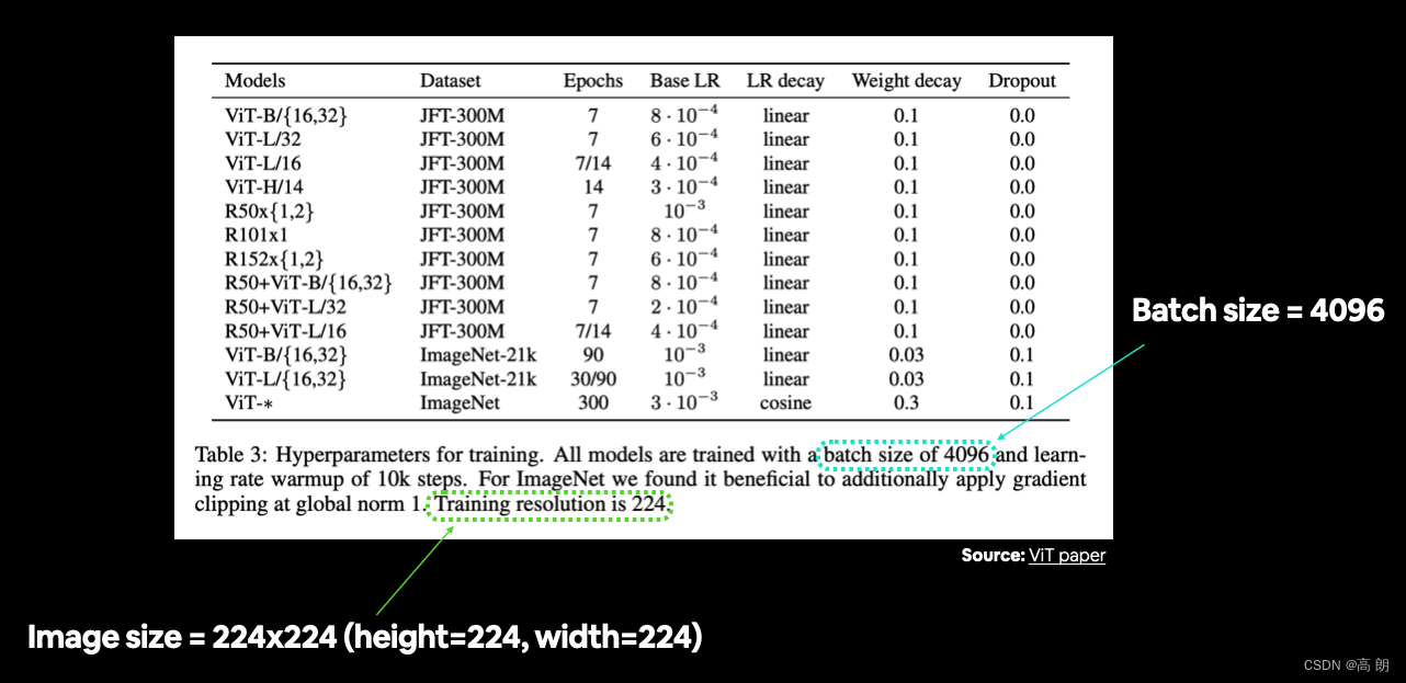
根据论文中指出训练分辨率为224(高度=224,宽度=224)
- 准备图像转换
# Create image size (from Table 3 in the ViT paper)
IMG_SIZE = 224

# Create transform pipeline manually
manual_transforms = transforms.Compose([
    transforms.Resize((IMG_SIZE, IMG_SIZE)),
    transforms.ToTensor(),
])
print(f"Manually created transforms: {manual_transforms}")
- 将图像转为 DataLoader
ViT 论文指出使用 4096 的批量大小,但是自己的硬件无法支持这么大的,改为32。
# Set the batch size
BATCH_SIZE = 32 # this is lower than the ViT paper but it's because we're starting small

# Create data loaders
train_dataloader, test_dataloader, class_names = data_setup.create_dataloaders(
    train_dir=train_dir,
    test_dir=test_dir,
    transform=manual_transforms, # use manually created transforms
    batch_size=BATCH_SIZE
)

train_dataloader, test_dataloader, class_names
我们在
create_dataloaders()函数中使用pin_memory=True参数来加速计算。pin_memory=True通过“固定”以前见过的示例,避免了 CPU 和 GPU 内存之间不必要的内存 复现。尽管这种好处可能会在较大的数据集大小中体现出来(FoodVision Mini 数据集非常小)。然而,设置pin_memory=True并不总是能提高性能(这是我们在机器学习中的另一个场景,其中有些东西有时起作用,有时不起作用),所以最好不断地实验,实验。
- 可视化单个图像
查看单个图像及其标签
从一批数据中获取单个图像和标签并检查它们的形状:
# Get a batch of images
image_batch, label_batch = next(iter(train_dataloader))

# Get a single image from the batch
image, label = image_batch[0], label_batch[0]

# View the batch shapes
image.shape, label
(torch.Size([3, 224, 224]), tensor(2))
用 matplotlib 绘制图像及其标签:
# Plot image with matplotlib
plt.imshow(image.permute(1, 2, 0)) # rearrange image dimensions to suit matplotlib [color_channels, height, width] -> [height, width, color_channels]
plt.title(class_names[label])
plt.axis(False);

3. 复现 ViT 论文:概述
模型输入是:披萨、牛排和寿司的图像。
模型输出是:披萨、牛排或寿司的预测标签
- 输入和输出、层和块
ViT 是一种深度学习神经网络架构,任何神经网络架构通常都是由层layers组成的,层的集合通常称为块block。将许多块堆叠在一起就是整个架构的基础。
层接受输入(例如图像张量),对其执行某种功能(例如层的 forward() 方法中的内容),然后返回输出。
因此,如果单个层接受输入并给出输出,那么层的集合(块)也接受输入并给出输出。
layers ——接受输入,对其执行函数,返回输出
block ——层的集合,接受输入,对其执行一系列功能,返回输出。
architecture (or model)—— 块的集合,接受输入,对其执行一系列功能,返回输出。
为了更好地理解,将对其进行分解,从单层的输入和输出开始,一直到整个模型的输入和输出。
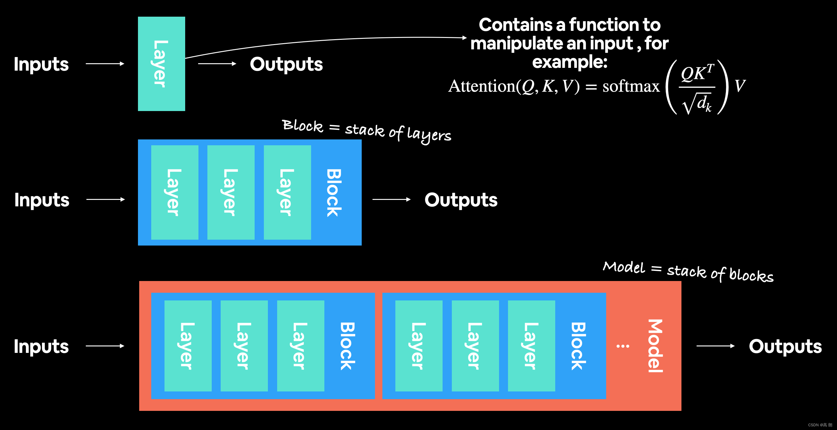 现在深度学习架构通常是层和块的集合。层接受输入(作为数字表示的数据)并使用某种函数对其进行操作(例如,上图所示的自注意力公式,但是,该函数几乎可以是任何东西),然后输出它。块通常是彼此堆叠的层,与单层执行类似的操作,但会执行多次。
- 具体来说:ViT 是由什么组成的
在架构设计中需要考虑的三个主要资源是:
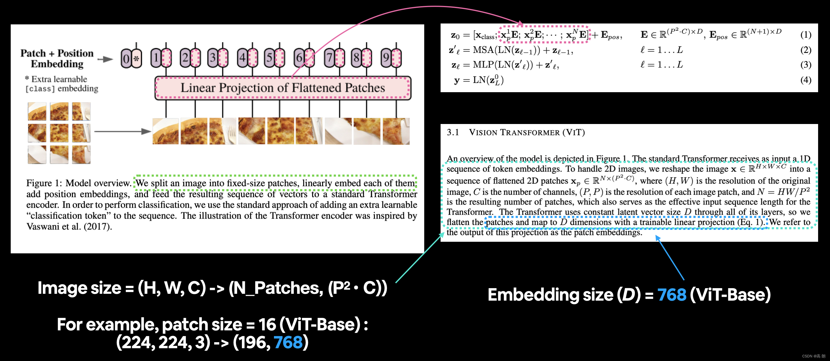
- Figure 1:从图形意义上给出了模型的概述,几乎可以仅使用此图重新创建架构。
- 四个公式:这些公式为图 1 中的彩色块提供了更多的数学基础。
- Table 1: 此表显示了不同 ViT 模型变体的各种超参数设置(例如层数和隐藏单元数)。重点关注最小的版本 ViT-Base。
Figure 1:
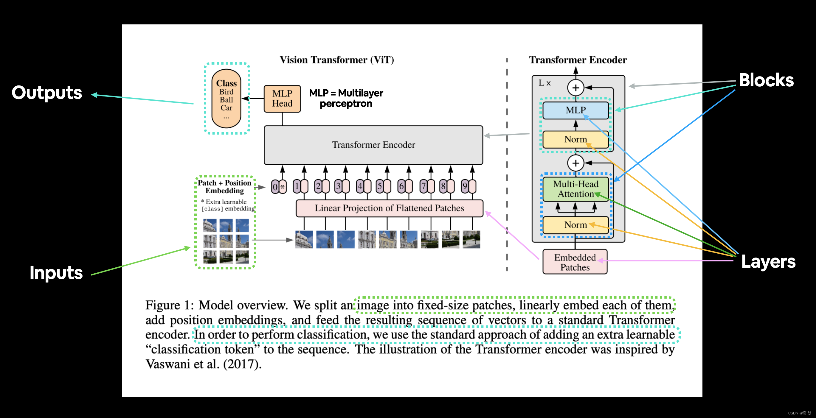 ViT 论文中的图 1 展示了创建架构的不同输入、输出、层和块。我们的目标是使用 PyTorch 代码 复现其中的每一个。
ViT 架构由几个阶段组成:
- Patch + Position Embedding (inputs):patch + 位置嵌入(输入)- 将输入图像转换为图像 patch 序列,并添加位置编号以指定 patch 出现的顺序。
- Linear projection of flattened patches (Embedded Patches):扁平化 patch 的线性投影(嵌入 patch ) - 图像 patch 变成嵌入,使用嵌入而不仅仅是图像值的好处是嵌入是可学习的表示(通常以向量的形式)通过训练可以改善的形象。
- Norm : 这是“Layer Normalization”或“LayerNorm”的缩写,是一种用于正则化(减少过度拟合)神经网络的技术,可以通过 PyTorch 层
torch.nn.LayerNorm()使用 LayerNorm 。 - Multi-Head Attention:多头注意力,这是多头自注意力层或简称“MSA”。可以通过 PyTorch 层
torch.nn.MultiheadAttention()创建 MSA 层。 - MLP (or Multilayer perceptron):MLP(或多层感知器),MLP 通常可以指任何前馈层的集合(或者在 PyTorch 的情况下,是具有 forward() 方法的层的集合)。在 ViT 论文中,作者将 MLP 称为“MLP 块”,它包含两个
torch.nn.Linear()层,它们之间有一个torch.nn.GELU()非线性激活和一个每个之后的torch.nn.Dropout()层。 - Transformer Encoder:Transformer 编码器 ,Transformer 编码器是上面列出的层的集合。 Transformer 编码器内部有两个跳跃连接(“+”符号),这意味着该层的输入直接馈送到直接层以及后续层。整个 ViT 架构由多个堆叠在一起的 Transformer 编码器组成。
- MLP Head:这是架构的输出层,它将输入的学习特征转换为类输出。由于我们正在研究图像分类,因此也可以将其称为“分类器头”。 MLP Head的结构与MLP块类似。
四个公式:
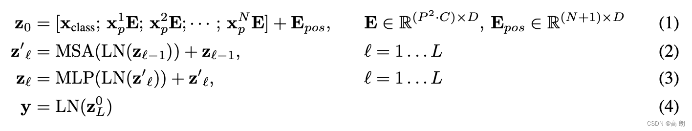 这四个公式代表了 ViT 架构四个主要部分背后的数学原理。
| Equation number | Description from ViT paper section 3.1 |
|---|---|
| 1 | …Transformer 在其所有层中使用恒定的潜在向量大小 D D D_D DD ,因此我们将 patch 展平并映射到 D D D_D DD |
| 2 | Transformer 编码器(Vaswani 等人,2017)由多头自注意力(MSA,参见附录 A)和 MLP 块(公式 2、3)的交替层组成。 Layernorm (LN) 应用在每个块之前,并在每个块之后应用残差连接(Wang et al., 2019;Baevski & Auli, 2019)。 |
| 3 | 与公式 2 相同。 |
| 4 | 与 BERT 的 [ class ] token 类似,我们在嵌入 patch 序列 ( z 00 = x c l a s s ) ( z 00 = x c l a s s ) (z_{00}=x_{class} )_{ (z_{00}=x_{class} )} (z00=xclass)(z00=xclass) 前面添加一个可学习的嵌入,其状态位于 Transformer 编码器的输出 ( z 0 L ) ( z 0 L ) (z_{0L})_ {(z_{0L})} (z0L)(z0L) 用作图像表示 y (公式 4)… |
映射到图 1 中的 ViT 架构:
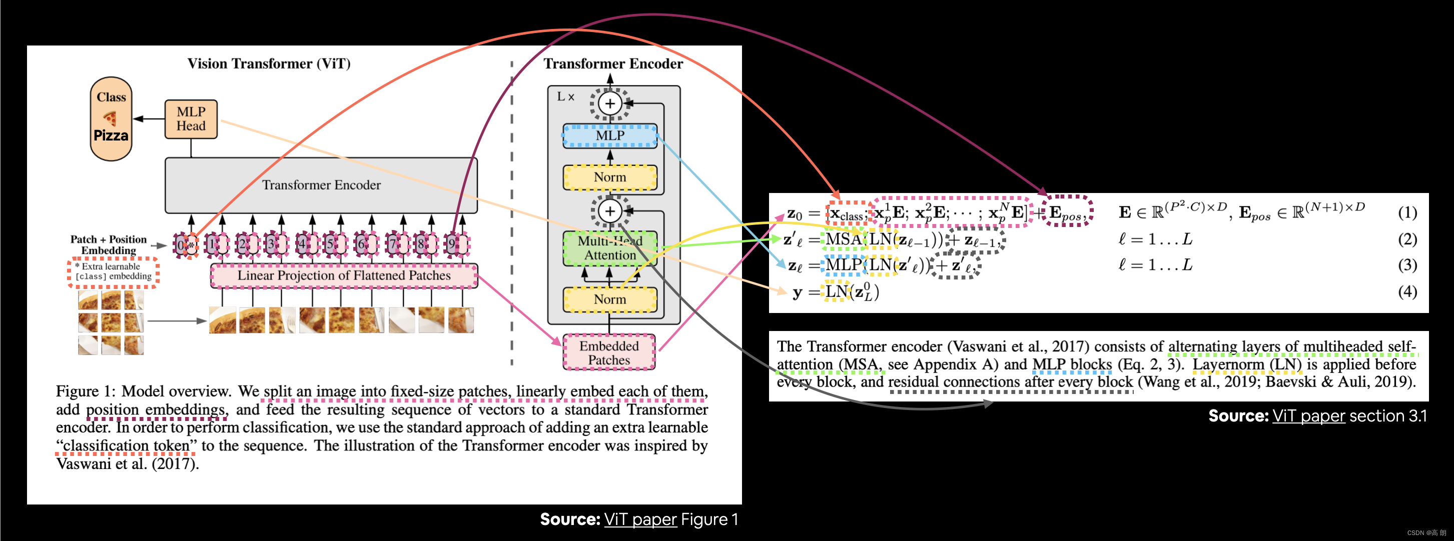
在所有公式(公式 4 除外)中,“ z ”是特定层的原始输出:

- z 0 z_0 z0 这是初始 patch 嵌入层的输出.
- z ℓ ′ z^′_ℓ zℓ′ 是“特定层素数的 z”(或 z 的中间值)
- z ℓ z_ℓ zℓ 是“特定层的 z”
y 是架构的整体输出。
公式1:
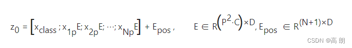 该公式处理输入图像的 class token 、 patch 嵌入和位置嵌入( E 用于嵌入)。
在向量形式中,嵌入可能类似于:
x_input = [class_token, image_patch_1, image_patch_2, image_patch_3...] + [class_token_position, image_patch_1_position, image_patch_2_position, image_patch_3_position...]
向量中的每个元素都是可学习的(它们的 requires_grad=True )。
公式2:
 这表示从 1 到 L (总层数)的每一层,都有一个多头注意力层 (MSA) 包裹着 LayerNorm 层 (LN)。
末尾的加法相当于将输入与输出相加,形成skip/residual连接。
将此层称为MSA 块。
在伪代码中,这可能看起来像:
x_output_MSA_block = MSA_layer(LN_layer(x_input)) + x_input
请注意末尾的 skip 连接(将层的输入添加到层的输出)。
公式3:
这表示对于从 1 到 L (总层数)的每一层,还有一个多层感知器层(MLP)包裹着 LayerNorm 层(LN)。
最后的添加显示了 skip/residual 连接的存在。
将这一层称为“MLP 块”。
在伪代码中,这可能看起来像:
x_output_MLP_block = MLP_layer(LN_layer(x_output_MSA_block)) + x_output_MSA_block
请注意末尾的skip连接(将层的输入添加到层的输出)。
公式4:
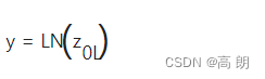 这表示对于最后一层 L ,输出 y 是 z 的 0 索引标记 包裹在 LayerNorm 层 (LN) 中。
x_output_MLP_block 的 0 索引:y = Linear_layer(LN_layer(x_output_MLP_block[0]))
表1: ViT论文中的Table 1
| Model | Layers | Hidden size D | MLP size | Heads | Params |
|---|---|---|---|---|---|
| ViT-Base | 12 | 768 | 3072 | 12 | 86M |
| ViT-Large | 24 | 1024 | 4096 | 16 | 307M |
| ViT-Huge | 32 | 1280 | 5120 | 16 | 632M |
表 1:Vision Transformer 模型变体的详细信息。资料来源:ViT 论文
本文将专注于复现 ViT-Base(从小规模开始,必要时扩大规模),但我们将编写可以轻松扩展到更大变体的代码。
分解超参数:
- Layers:有多少个 Transformer Encoder 块? (其中每个都包含一个 MSA 块和 MLP 块)
- Hidden size D: 这是整个架构中的嵌入维度,这将是我们的图像在修补和嵌入时变成的向量的大小。一般来说,嵌入维数越大,可以捕获的信息越多,结果越好。然而,更大的嵌入是以更多计算为代价的。
- MLP size:MLP 层中隐藏单元的数量是多少?
- Heads:多头注意力层中有多少个头?
- Params:模型的参数总数是多少?一般来说,更多的参数会带来更好的性能,但代价是更多的计算。 会注意到,甚至 ViT-Base 的参数也比我们迄今为止使用的任何其他模型都要多得多。
- 复现论文的工作流程
(1)从头到尾阅读整篇论文一次(以了解主要概念)。
(2)回顾每个部分,看看它们如何相互配合,并开始思考如何将它们转化为代码(就像上面一样)。
(3)重复步骤 2,直到获得相当好的提纲/思路。
(4)使用 mathpix.com(一个非常方便的工具)将论文的任何部分转换为 markdown/LaTeX 以放入笔记本中。
(5)尽可能 复现模型的最简单版本。
(6)如果遇到困难,查找其他示例。
附使用 mathpix.com 将 ViT 论文中的四个公式转换为可编辑的 LaTeX/markdown:

4. Equation 1: 将数据拆分为 patch 并创建类、位置和 patch 嵌入
【以一种良好的、可学习的方式表示你的数据(因为嵌入是可学习的表示),那么学习算法很可能能够在它们上表现良好。】
首先为 ViT 架构创建类、位置和 patch 嵌入。
从 patch 嵌入开始,这意味着我们将把输入图像转换为一系列 patch ,然后嵌入这些 patch 。
嵌入是某种形式的可学习表示,并且通常是向量。
“可学习”一词很重要,因为这意味着输入图像(模型看到的)的数字表示可以随着时间的推移而得到改进。
标准 Transformer 接收一维令牌嵌入序列作为输入。为了处理 2D 图像,我们将图像 x ∈ R H × W × C x \in R^{H \times W \times C} x∈RH×W×C 重塑为一系列扁平的 2D patch x p ∈ R N × ( P 2 ⋅ C ) x_p \in R^{N \times\left(P^2 \cdot C\right)} xp∈RN×(P2⋅C) ,其中 (H,W) 为原图分辨率, C 为通道数, (P,P) 是生成的块数量,它也作为Transformer的有效输入序列长度。 Transformer在其所有层中使用恒定的潜在向量大小D,因此我们将 patch 展平,并使用可训练的线性投影将其映射到D维空间(公式1)。我们将该投影的输出称为 patch 嵌入。
我们处理图像形状的尺寸,让我们记住 ViT 论文表 3 中的一行:训练分辨率为224。
分解一下上面的文字:
- D 是 patch 嵌入的大小,不同大小的 ViT 模型的 D 的不同值可以在表 1 中找到。
- 图像以 2D 形式开始,大小为 H×W×C 。
- 图像被转换为大小为 N × ( P 2 ⋅ C ) N \times\left(P^2 \cdot C\right) N×(P2⋅C) 的扁平 2D patch 序列。【(P,P) 是每个图像块的分辨率(块大小)。】【 N = H W / P 2 N=HW/P^2 N=HW/P2 是生成的 patch 数量,它也用作 Transformer 的输入序列长度】
将 ViT 架构的 patch 和位置嵌入部分从图 1 映射到公式 1。第 3.1 节的开头段落描述了 patch 嵌入层的不同输入和输出形状。
- 手动计算 patch 嵌入输入和输出形状
使用 16 的 patch 大小 ( P ),因为它是 ViT-Base 使用的最佳性能版本(请参见表 5 中的“ViT-B/16”列)
# Create example values
height = 224 # H ("The training resolution is 224.")
width = 224 # W
color_channels = 3 # C
patch_size = 16 # P

# Calculate N (number of patches)
number_of_patches = int((height * width) / patch_size**2)
print(f"Number of patches (N) with image height (H={height}), width (W={width}) and patch size (P={patch_size}): {number_of_patches}")
Number of patches (N) with image height (H=224), width (W=224) and patch size (P=16): 196
得到图片块patches的大小,即生成的patch数:196
开始 复现 patches 嵌入层的输入和输出形状:
- input : 图像以 2D 形式开始,大小为 H×W×C
- Output:图像被转换为大小为 N × ( P 2 ⋅ C ) N \times\left(P^2 \cdot C\right) N×(P2⋅C) 的扁平 2D patch序列。
# Input shape (this is the size of a single image)
embedding_layer_input_shape = (height, width, color_channels)

# Output shape
embedding_layer_output_shape = (number_of_patches, patch_size**2 * color_channels)

print(f"Input shape (single 2D image): {embedding_layer_input_shape}")
print(f"Output shape (single 2D image flattened into patches): {embedding_layer_output_shape}")
Input shape (single 2D image): (224, 224, 3)
Output shape (single 2D image flattened into patches): (196, 768)
- 将单个图像变成 patches图像块
正在做的是将整体架构分解为更小的部分,重点关注各个层的输入和输出。
如何创建 patch 嵌入层:
从单张图片开始:
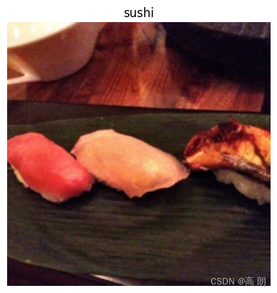
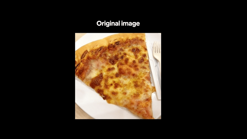
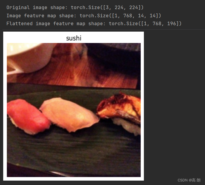
# View single image
plt.imshow(image.permute(1, 2, 0)) # adjust for matplotlib
plt.title(class_names[label])
plt.axis(False);
希望将此图像转换为与 ViT 论文的图 1 一致的图像块:
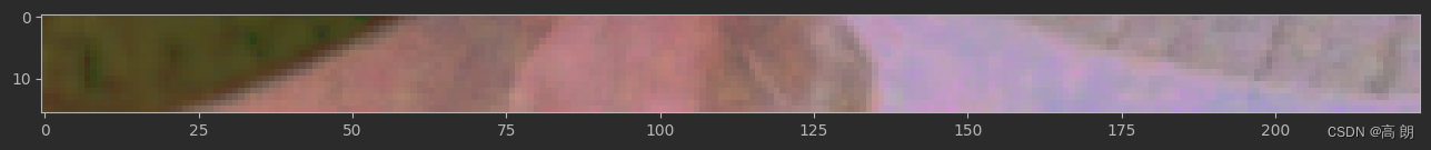
先从仅可视化 patch 像素的顶行开始:(可以通过在不同的图像尺寸上建立索引来做到这一点)
# Change image shape to be compatible with matplotlib (color_channels, height, width) -> (height, width, color_channels)
image_permuted = image.permute(1, 2, 0)

# Index to plot the top row of patched pixels
patch_size = 16
plt.figure(figsize=(patch_size, patch_size))
plt.imshow(image_permuted[:patch_size, :, :]);
现在已经得到了顶行,让我们把它变成 patches:(可以通过迭代顶行中的 patch 数量来做到这一点)
# Setup hyperparameters and make sure img_size and patch_size are compatible
img_size = 224
patch_size = 16
num_patches = img_size/patch_size
assert img_size % patch_size == 0, "Image size must be divisible by patch size"
print(f"Number of patches per row: {num_patches}\nPatch size: {patch_size} pixels x {patch_size} pixels")

# Create a series of subplots
fig, axs = plt.subplots(nrows=1,
                        ncols=img_size // patch_size, # one column for each patch
                        figsize=(num_patches, num_patches),
                        sharex=True,
                        sharey=True)

# Iterate through number of patches in the top row
for i, patch in enumerate(range(0, img_size, patch_size)):
    axs[i].imshow(image_permuted[:patch_size, patch:patch+patch_size, :]); # keep height index constant, alter the width index
    axs[i].set_xlabel(i+1) # set the label
    axs[i].set_xticks([])
    axs[i].set_yticks([])
Number of patches per row: 14.0
Patch size: 16 pixels x 16 pixels
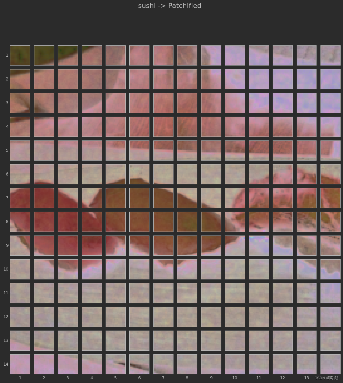
 开始对整个图像进行处理:(将迭代高度和宽度的索引,并将每个 patch绘制为它自己的子图)
# Setup hyperparameters and make sure img_size and patch_size are compatible
img_size = 224
patch_size = 16
num_patches = img_size/patch_size
assert img_size % patch_size == 0, "Image size must be divisible by patch size"
print(f"Number of patches per row: {num_patches}\
        \nNumber of patches per column: {num_patches}\
        \nTotal patches: {num_patches*num_patches}\
        \nPatch size: {patch_size} pixels x {patch_size} pixels")

# Create a series of subplots
fig, axs = plt.subplots(nrows=img_size // patch_size, # need int not float
                        ncols=img_size // patch_size,
                        figsize=(num_patches, num_patches),
                        sharex=True,
                        sharey=True)

# Loop through height and width of image
for i, patch_height in enumerate(range(0, img_size, patch_size)): # iterate through height
    for j, patch_width in enumerate(range(0, img_size, patch_size)): # iterate through width

        # Plot the permuted image patch (image_permuted -> (Height, Width, Color Channels))
        axs[i, j].imshow(image_permuted[patch_height:patch_height+patch_size, # iterate through height
                                        patch_width:patch_width+patch_size, # iterate through width
                                        :]) # get all color channels

        # Set up label information, remove the ticks for clarity and set labels to outside
        axs[i, j].set_ylabel(i+1,
                             rotation="horizontal",
                             horizontalalignment="right",
                             verticalalignment="center")
        axs[i, j].set_xlabel(j+1)
        axs[i, j].set_xticks([])
        axs[i, j].set_yticks([])
        axs[i, j].label_outer()

# Set a super title
fig.suptitle(f"{class_names[label]} -> Patchified", fontsize=16)
plt.show()
Number of patches per row: 14.0
Number of patches per column: 14.0
Total patches: 196.0
Patch size: 16 pixels x 16 pixels
 后续需要考虑的是如何将每个 patch 转换为嵌入并将它们转换为序列。
- 使用
torch.nn.Conv2d()创建图像 patches
已经看到了图像变成 patches 时的样子,开始使用 PyTorch 复现 patch
embedding layers
ViT 论文的作者在第 3.1 节中提到,patch 嵌入可以通过卷积神经网络(CNN)来实现:
Hybrid Architecture. 作为原始图像块的替代方案,输入序列可以由 CNN 的特征图形成(LeCun 等人,1989)。在此混合模型中,patch 嵌入投影 E (公式 1)应用于从 CNN 特征图中提取的 patch 。作为一种特殊情况, patch 可以具有空间大小 1×1 ,这意味着输入序列是通过简单地展平特征图的空间维度并投影到 Transformer 维度来获得的。如上所述添加分类输入嵌入和位置嵌入。
“特征图”是卷积层经过给定图像时产生的权重/激活。
通过将 torch.nn.Conv2d() 图层的 kernel_size 和 stride 参数设置为等于 patch_size ,我们可以有效地获得一个分割图像的图层成 patch 并为每个 patch 创建一个可学习的嵌入(在 ViT 论文中称为“线性投影”)。
对于图像大小为 224 且块大小(patch_size)为 16 的情况:
Input (2D image):(224, 224, 3) -> (height, width, color channels)Output (flattened 2D patches):(196, 768) -> (number of patches, embedding dimension)
可以通过以下方式重新创建它们:
torch.nn.Conv2d()用于将我们的图像转换为 CNN 特征图块。torch.nn.Flatten()用于展平特征图的空间维度。
关于torch.nn.Conv2d() 层处理:
可以通过将 kernel_size 和 stride 设置为 patch_size 来复现 patch 的创建。
这意味着每个卷积核的大小将为 (patch_size x patch_size) 或 patch_size=16 、 (16 x 16) (相当于一个完整的 patch)。
卷积核的每个步长或 stride 将是 patch_size 像素长或 16 像素长(相当于步进到下一个patch)。
设置 in_channels=3 作为图像中颜色通道的数量,并设置 out_channels=768 ,与 表 1 中 ViT-Base 的值(这是嵌入维度,每个图像将被嵌入到大小为 768 的可学习向量中)。
from torch import nn

# Set the patch size
patch_size=16

# Create the Conv2d layer with hyperparameters from the ViT paper
conv2d = nn.Conv2d(in_channels=3, # number of color channels
                   out_channels=768, # from Table 1: Hidden size D, this is the embedding size
                   kernel_size=patch_size, # could also use (patch_size, patch_size)
                   stride=patch_size,
                   padding=0)
有了一个卷积层,测试将单个图像传递给它时会发生什么:
原图片:
# View single image
plt.imshow(image.permute(1, 2, 0)) # adjust for matplotlib
plt.title(class_names[label])
plt.axis(False);

卷积操作:
# Pass the image through the convolutional layer
image_out_of_conv = conv2d(image.unsqueeze(0)) # add a single batch dimension (height, width, color_channels) -> (batch, height, width, color_channels)
print(image_out_of_conv.shape)
torch.Size([1, 768, 14, 14])
将图像通过卷积层将其变成一系列 768 个(这是嵌入大小或 D )特征/激活图。torch.Size([1, 768, 14, 14]) -> [batch_size, embedding_dim, feature_map_height, feature_map_width]
可视化五个随机特征图,看看它们是什么样子的:
# Plot random 5 convolutional feature maps
import random
random_indexes = random.sample(range(0, 758), k=5) # pick 5 numbers between 0 and the embedding size
print(f"Showing random convolutional feature maps from indexes: {random_indexes}")

# Create plot
fig, axs = plt.subplots(nrows=1, ncols=5, figsize=(12, 12))

# Plot random image feature maps
for i, idx in enumerate(random_indexes):
    image_conv_feature_map = image_out_of_conv[:, idx, :, :] # index on the output tensor of the convolutional layer
    axs[i].imshow(image_conv_feature_map.squeeze().detach().numpy())
    axs[i].set(xticklabels=[], yticklabels=[], xticks=[], yticks=[]);
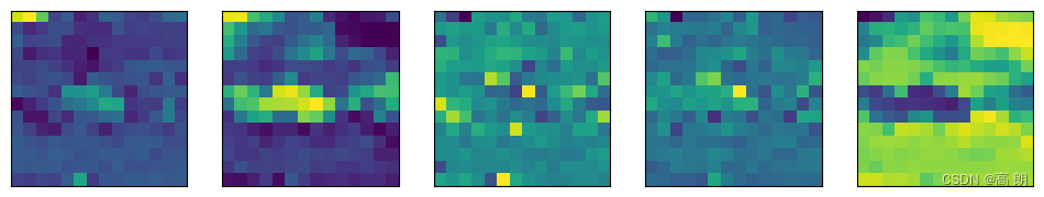 注意特征图如何代表原始图像,在可视化更多之后, 可以开始看到不同的主要轮廓和一些主要特征
需要注意的重要一点是,随着神经网络的学习,这些特征可能会随着时间的推移而改变。正因为如此,这些特征图可以被认为是我们图像的可学习嵌入。
数字形式检查一下:
# Get a single feature map in tensor form
single_feature_map = image_out_of_conv[:, 0, :, :]
single_feature_map, single_feature_map.requires_grad
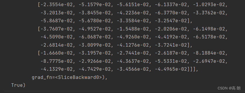
single_feature_map 和 requires_grad=True 属性的 grad_fn 输出意味着 PyTorch 正在跟踪该特征图的梯度,并且它将在训练期间通过梯度下降进行更新。
- 使用
torch.nn.Flatten()压平 patch 嵌入
已经将图像转换为 patch 嵌入,但它们仍然是 2D 格式,如何将它们变成 ViT 模型的 patch 嵌入层所需的输出形状,所需输出(展平 2D patch 的 1D 序列): (196, 768) -> ( patch 数量,嵌入维度) -> N × ( P 2 ⋅ C ) N×(P^2⋅C) N×(P2⋅C)。
当前的形状:
# Current tensor shape
print(f"Current tensor shape: {image_out_of_conv.shape} -> [batch, embedding_dim, feature_map_height, feature_map_width]")
Current tensor shape: torch.Size([1, 768, 14, 14]) -> [batch, embedding_dim, feature_map_height, feature_map_width]
已经得到了 768 部分( ( P 2 ⋅ C P^2⋅C P2⋅C) ),但我们仍然需要 patch 的数量( N )。
回顾一下 ViT 论文的第 3.1 节:作为一种特殊情况,patch 可以具有空间大小 1×1 ,这意味着输入序列是通过简单地展平特征图的空间维度并投影到 Transformer 维度来获得的。
不想展平整个张量,我们只想展平“特征图的空间维度”,在我们的例子中,是 image_out_of_conv 的 feature_map_height 和 feature_map_width 尺寸。
创建一个 torch.nn.Flatten() 图层来仅展平这些尺寸,我们可以使用 start_dim 和 end_dim 参数来设置它:
# Create flatten layer
flatten = nn.Flatten(start_dim=2, # flatten feature_map_height (dimension 2)
                     end_dim=3) # flatten feature_map_width (dimension 3)
可以将其组合到一起了,在这之前回顾一下流程:
(1)获取一张图片
(2)通过卷积层( conv2d )放入,将图像转换为 2D 特征图(patch嵌入)
(3)将 2D 特征图展平为单个序列
# 1. View single image
plt.imshow(image.permute(1, 2, 0)) # adjust for matplotlib
plt.title(class_names[label])
plt.axis(False);
print(f"Original image shape: {image.shape}")

# 2. Turn image into feature maps
image_out_of_conv = conv2d(image.unsqueeze(0)) # add batch dimension to avoid shape errors
print(f"Image feature map shape: {image_out_of_conv.shape}")

# 3. Flatten the feature maps
image_out_of_conv_flattened = flatten(image_out_of_conv)
print(f"Flattened image feature map shape: {image_out_of_conv_flattened.shape}")
当前形状:(1, 768, 196)
所需: (196, 768) ->
N
×
(
P
2
⋅
C
)
N×(P^2⋅C)
N×(P2⋅C)
唯一的区别是当前的形状具有批量大小,并且尺寸与所需输出的顺序不同。
以使用 torch.Tensor.permute() 来实现这一点,就像重新排列图像张量以使用 matplotlib 绘制它们一样。
# Get flattened image patch embeddings in right shape
image_out_of_conv_flattened_reshaped = image_out_of_conv_flattened.permute(0, 2, 1) # [batch_size, P^2•C, N] -> [batch_size, N, P^2•C]
print(f"Patch embedding sequence shape: {image_out_of_conv_flattened_reshaped.shape} -> [batch_size, num_patches, embedding_size]")
Patch embedding sequence shape: torch.Size([1, 196, 768]) -> [batch_size, num_patches, embedding_size]
现在,已经使用几个 PyTorch 层为 ViT 架构的 patch 嵌入层匹配了所需的输入和输出形状。
可视化其中一张扁平化的特征图:
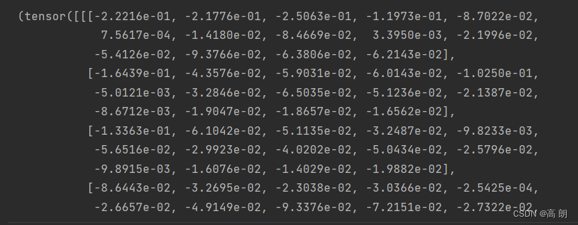
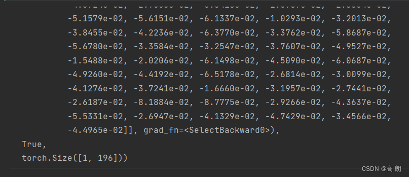
# Get a single flattened feature map
single_flattened_feature_map = image_out_of_conv_flattened_reshaped[:, :, 0] # index: (batch_size, number_of_patches, embedding_dimension)

# Plot the flattened feature map visually
plt.figure(figsize=(22, 22))
plt.imshow(single_flattened_feature_map.detach().numpy())
plt.title(f"Flattened feature map shape: {single_flattened_feature_map.shape}")
plt.axis(False);

扁平化的特征图在视觉上看起来不太像,但这不是我们关心的,这就是patch 嵌入层的输出和 ViT 架构其余部分的输入。
注意:最初的 Transformer 架构是为处理文本而设计的。 Vision Transformer 架构 (ViT) 的目标是使用原始 Transformer 来处理图像。这就是为什么 ViT 架构的输入按原样进行处理的原因。我们本质上是获取 2D 图像并对其进行格式化,使其显示为 1D 文本序列。
以张量形式查看扁平化的特征图:
# See the flattened feature map as a tensor
single_flattened_feature_map, single_flattened_feature_map.requires_grad, single_flattened_feature_map.shape
 现在,已将单个 2D 图像转换为 1D 可学习嵌入向量(或 ViT 论文图 1 中的“扁平化图像块的线性投影”)
- 将ViT patch 嵌入层变成PyTorch模块
可以通过子类化 nn.Module 并创建一个小型 PyTorch“模型”来完成,具体操作步骤如下:
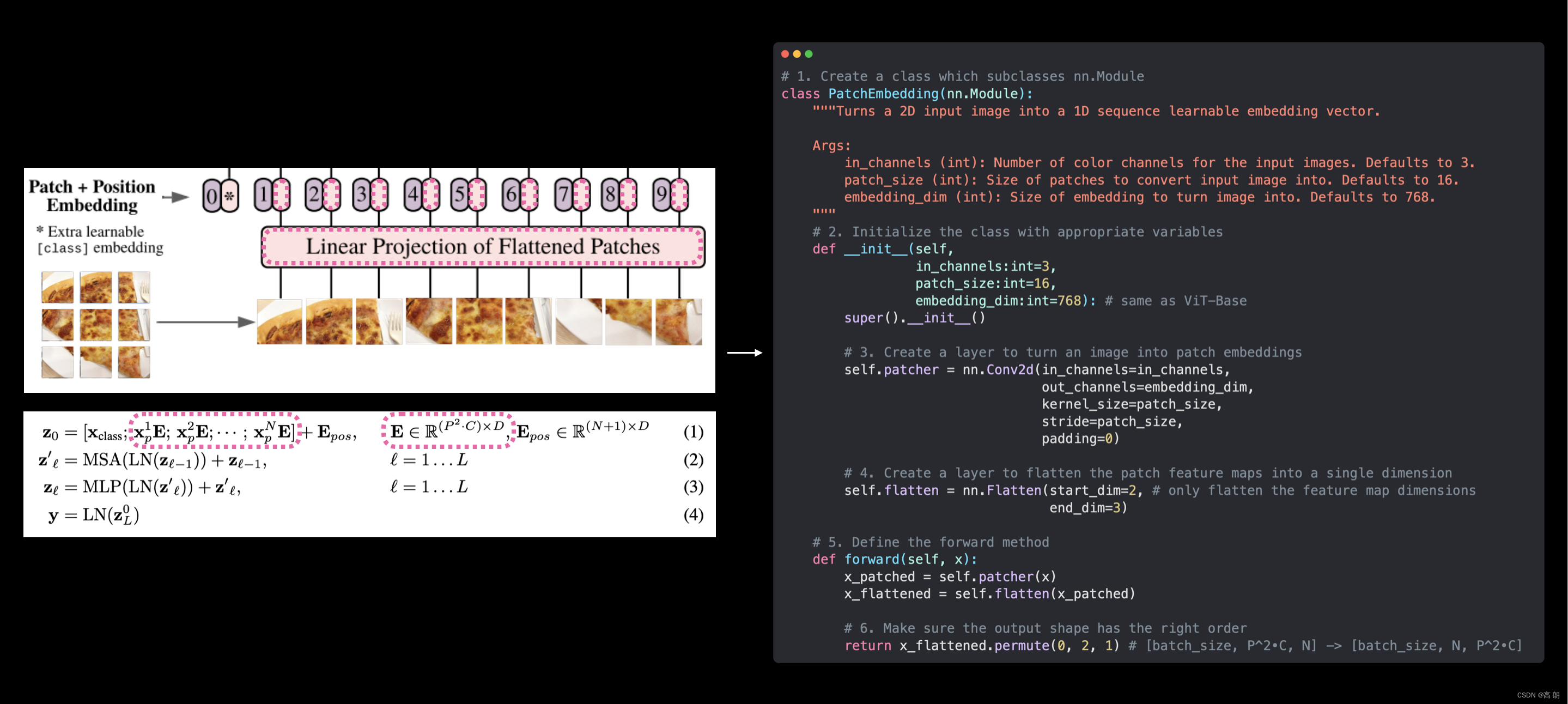
(1)创建一个名为 PatchEmbedding 的类,它是 nn.Module 的子类(因此可以将其用作 PyTorch 层)。
(2)使用参数 in_channels=3 、 patch_size=16 (对于 ViT-Base)和 embedding_dim=768 (这是
D
D
D_D
DD)
(3)使用 nn.Conv2d() 创建一个图层将图像转换为Patch 图像块。
(4)创建一个图层将 patch 特征图展平为单一维度。
(5)定义一个 forward() 方法来获取输入并将其传递到在 3 和 4 中创建的层。
(6)确保输出形状反映了 ViT 架构所需的输出形状
N
×
(
P
2
⋅
C
)
N×(P^2⋅C)
N×(P2⋅C)
# 1. Create a class which subclasses nn.Module
class PatchEmbedding(nn.Module):
    """Turns a 2D input image into a 1D sequence learnable embedding vector.

    Args:
        in_channels (int): Number of color channels for the input images. Defaults to 3.
        patch_size (int): Size of patches to convert input image into. Defaults to 16.
        embedding_dim (int): Size of embedding to turn image into. Defaults to 768.
    """
    # 2. Initialize the class with appropriate variables
    def __init__(self,
                 in_channels:int=3,
                 patch_size:int=16,
                 embedding_dim:int=768):
        super().__init__()

        # 3. Create a layer to turn an image into patches
        self.patcher = nn.Conv2d(in_channels=in_channels,
                                 out_channels=embedding_dim,
                                 kernel_size=patch_size,
                                 stride=patch_size,
                                 padding=0)

        # 4. Create a layer to flatten the patch feature maps into a single dimension
        self.flatten = nn.Flatten(start_dim=2, # only flatten the feature map dimensions into a single vector
                                  end_dim=3)

    # 5. Define the forward method
    def forward(self, x):
        # Create assertion to check that inputs are the correct shape
        image_resolution = x.shape[-1]
        assert image_resolution % patch_size == 0, f"Input image size must be divisble by patch size, image shape: {image_resolution}, patch size: {patch_size}"

        # Perform the forward pass
        x_patched = self.patcher(x)
        x_flattened = self.flatten(x_patched)
        # 6. Make sure the output shape has the right order
        return x_flattened.permute(0, 2, 1) # adjust so the embedding is on the final dimension [batch_size, P^2•C, N] -> [batch_size, N, P^2•C]
测试单个图像:
set_seeds()

# Create an instance of patch embedding layer
patchify = PatchEmbedding(in_channels=3,
                          patch_size=16,
                          embedding_dim=768)

# Pass a single image through
print(f"Input image shape: {image.unsqueeze(0).shape}")
patch_embedded_image = patchify(image.unsqueeze(0)) # add an extra batch dimension on the 0th index, otherwise will error
print(f"Output patch embedding shape: {patch_embedded_image.shape}")
Input image shape: torch.Size([1, 3, 224, 224])
Output patch embedding shape: torch.Size([1, 196, 768])
输出形状与我们希望从Patch嵌入层看到的理想输入和输出形状相匹配。
现在已经 复现了公式 1 的Patch嵌入,但没有复现class token 和 位置嵌入。
 PatchEmbedding 类(右) 复现了图 1 中 ViT 架构的Patch嵌入以及 ViT 论文(左)中的公式 1。然而,可学习的class token嵌入和位置嵌入尚未创建。
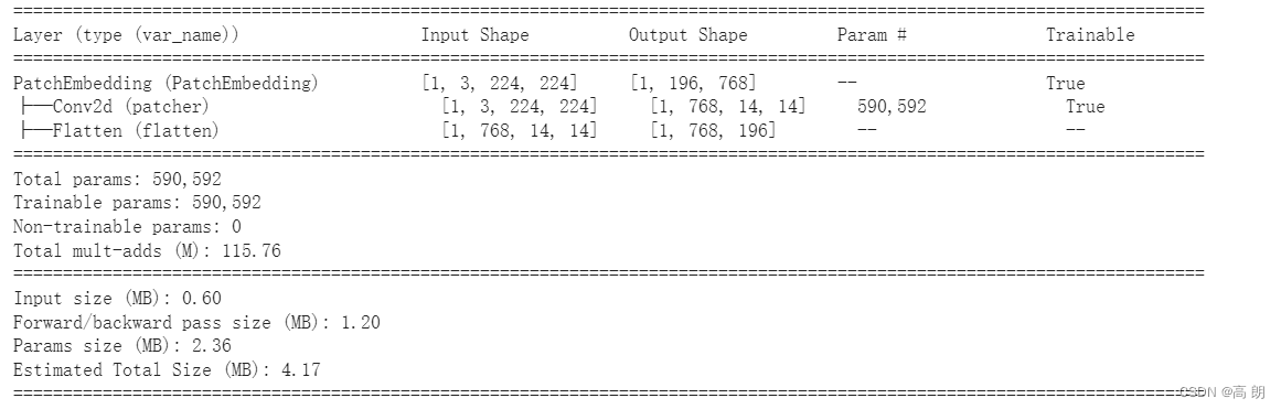
先用summary()总结一下 PatchEmbedding 层:
# Create random input sizes
random_input_image = (1, 3, 224, 224)
random_input_image_error = (1, 3, 250, 250) # will error because image size is incompatible with patch_size

# # Get a summary of the input and outputs of PatchEmbedding (uncomment for full output)
summary(PatchEmbedding(),
        input_size=random_input_image, # try swapping this for "random_input_image_error"
        col_names=["input_size", "output_size", "num_params", "trainable"],
        col_width=20,
        row_settings=["var_names"])
6. 创建class token embedding
公式 1 中的 x c l a s s x_{class} xclass
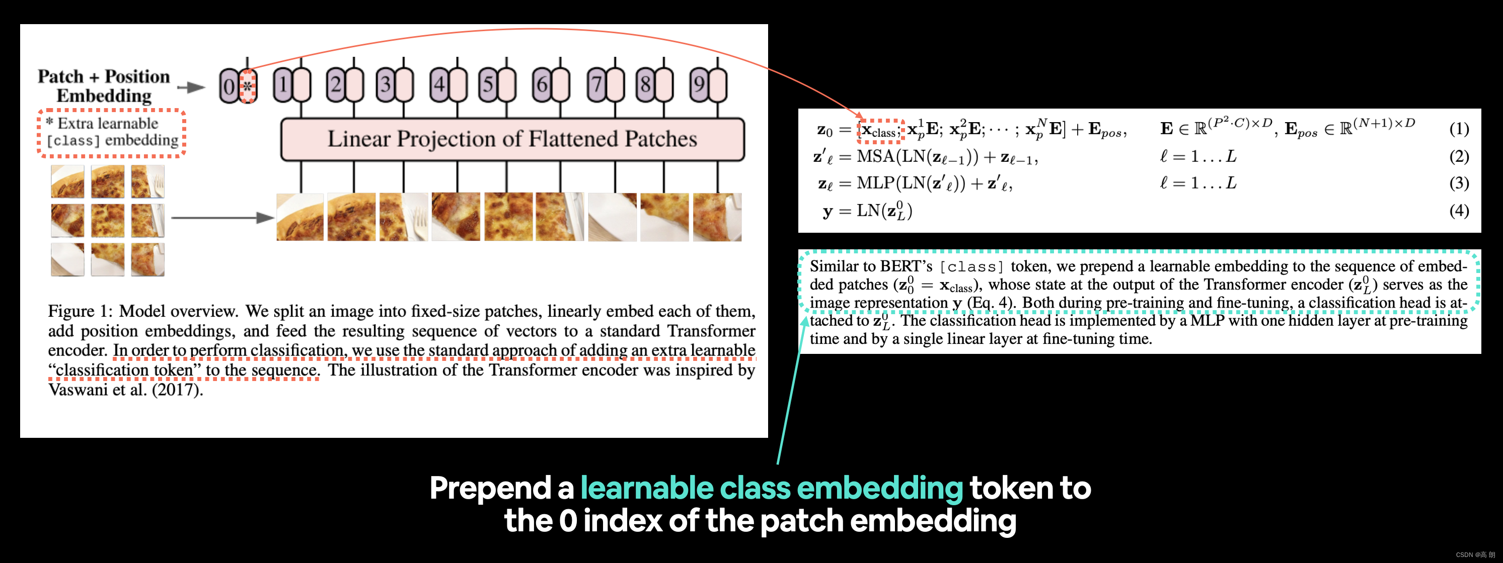 左:ViT 论文中的图 1,其中突出显示了我们将重新创建的“classification token”或 [class] 嵌入标记。右图:ViT 论文中与可学习class token 嵌入标记相关的公式 1 和第 3.1 节。
阅读ViT论文第3.1节第二段:
与 BERT 的 [ class ] 标记类似,我们在嵌入 patch 序列 ( z 00 = x c l a s s ) (z_{00}=x_{class} ) (z00=xclass)前面添加一个可学习的嵌入,其状态位于 Transformer 编码器的输出 ( z 0 L ) (z_{0L}) (z0L)用作图像表示 y y y(公式 4).
注:BERT(来自 Transformers 的双向编码器表示)是原始机器学习研究论文之一,旨在使用 Transformer 架构在自然语言处理 (NLP) 任务上取得出色的结果,并且正是 [ class ] 序列起始处的标记,class 是序列所属“classification ”类的描述。
因此,需要“在嵌入patch序列中预先准备一个可学习的嵌入”。
先查看嵌入Patch张量的序列(在 4.5 节中创建)及其形状:
# View the patch embedding and patch embedding shape
print(patch_embedded_image)
print(f"Patch embedding shape: {patch_embedded_image.shape} -> [batch_size, number_of_patches, embedding_dimension]")
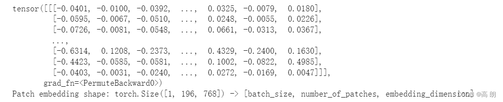 为了“将可学习的嵌入添加到嵌入Patch的序列中”,我们需要以 embedding_dimension ( D ) 的形式创建可学习的嵌入,然后将其添加到 number_of_patches 维度。
伪代码理解:
patch_embedding = [image_patch_1, image_patch_2, image_patch_3...]
class_token = learnable_embedding
patch_embedding_with_class_token = torch.cat((class_token, patch_embedding), dim=1)
串联 ( torch.cat() ) 发生在 dim=1 ( number_of_patches 维度)上。
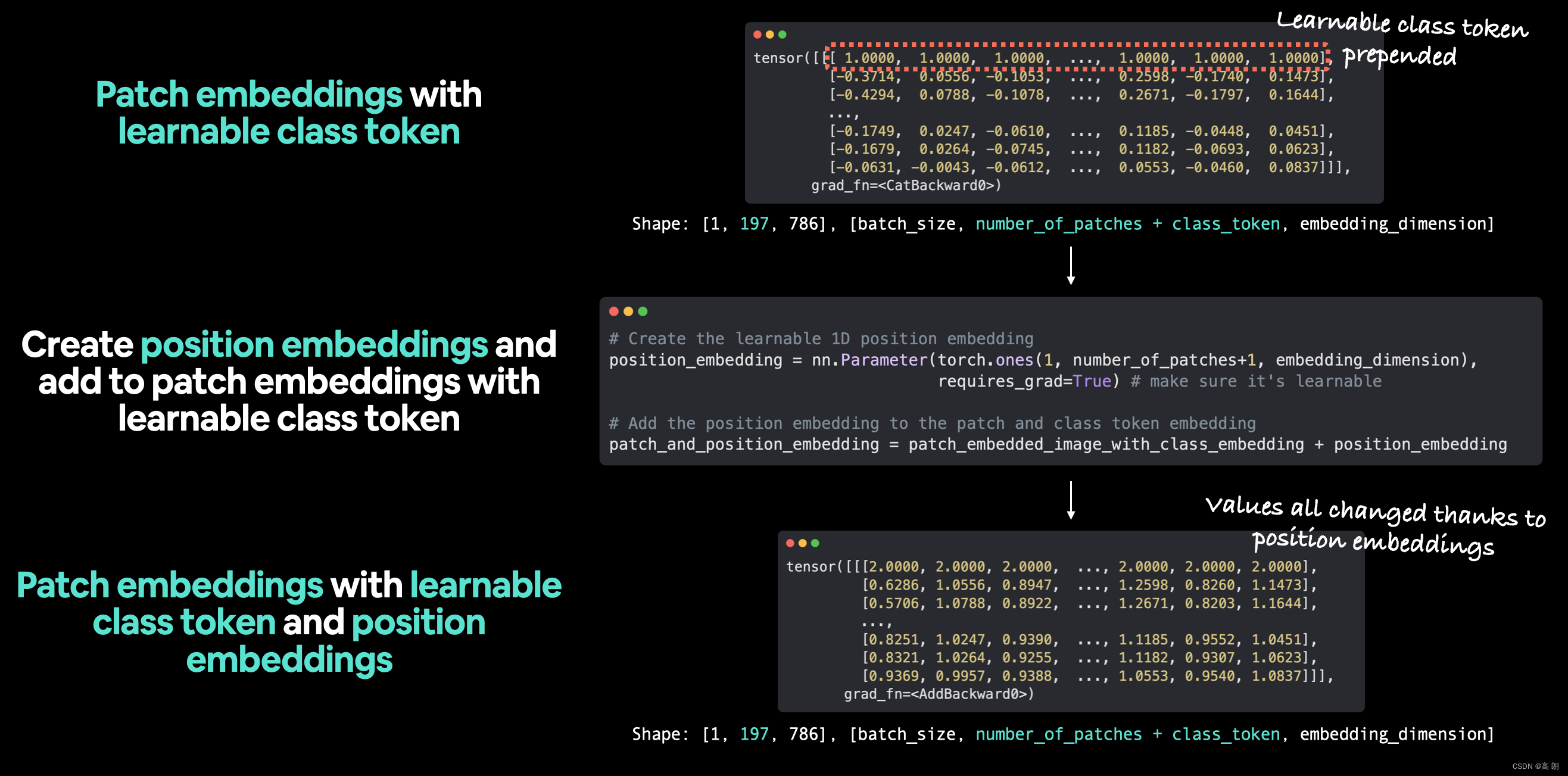
开始为class token创建一个可学习的嵌入:
获取批量大小和嵌入维度形状,然后以形状 [batch_size, 1, embedding_dimension] 创建一个 torch.ones() 张量。并过使用 requires_grad=True 将张量传递给 nn.Parameter() 来使张量变得可学习。
# Get the batch size and embedding dimension
batch_size = patch_embedded_image.shape[0]
embedding_dimension = patch_embedded_image.shape[-1]

# Create the class token embedding as a learnable parameter that shares the same size as the embedding dimension (D)
class_token = nn.Parameter(torch.ones(batch_size, 1, embedding_dimension), # [batch_size, number_of_tokens, embedding_dimension]
                           requires_grad=True) # make sure the embedding is learnable

# Show the first 10 examples of the class_token
print(class_token[:, :, :10])

# Print the class_token shape
print(f"Class token shape: {class_token.shape} -> [batch_size, number_of_tokens, embedding_dimension]")
tensor([[[1., 1., 1., 1., 1., 1., 1., 1., 1., 1.]]], grad_fn=<SliceBackward0>)
Class token shape: torch.Size([1, 1, 768]) -> [batch_size, number_of_tokens, embedding_dimension]
注意:在这里,我们仅将 class token 嵌入创建为 torch.ones() 以用于演示目的,实际上, 可能会使用 torch.randn() 创建 class token 嵌入(因为机器学习都是关于利用受控随机性的力量, 通常从随机数开始并随着时间的推移对其进行改进)。
class_token 的 number_of_tokens 维度是 1 ,因为我们只想在 patch 嵌入序列的开头添加一个class token 值。
现在已经获得了class token 嵌入,让我们将其添加到图像 patch 序列 patch_embedded_image 中:
可以使用 torch.cat() 并设置 dim=1 (因此 class_token 的 number_of_tokens 尺寸被预先考虑为 patch_embedded_image 的 number_of_patches 维度)。
# Add the class token embedding to the front of the patch embedding
patch_embedded_image_with_class_embedding = torch.cat((class_token, patch_embedded_image),
                                                      dim=1) # concat on first dimension

# Print the sequence of patch embeddings with the prepended class token embedding
print(patch_embedded_image_with_class_embedding)
print(f"Sequence of patch embeddings with class token prepended shape: {patch_embedded_image_with_class_embedding.shape} -> [batch_size, number_of_patches, embedding_dimension]")
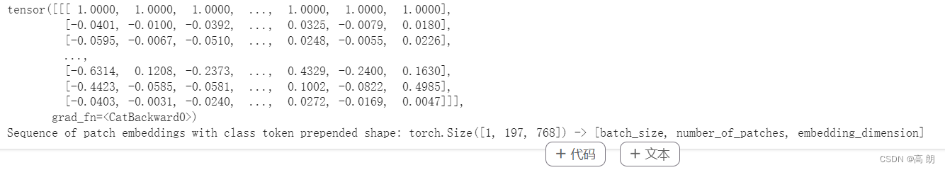 可学习的class token 前置:
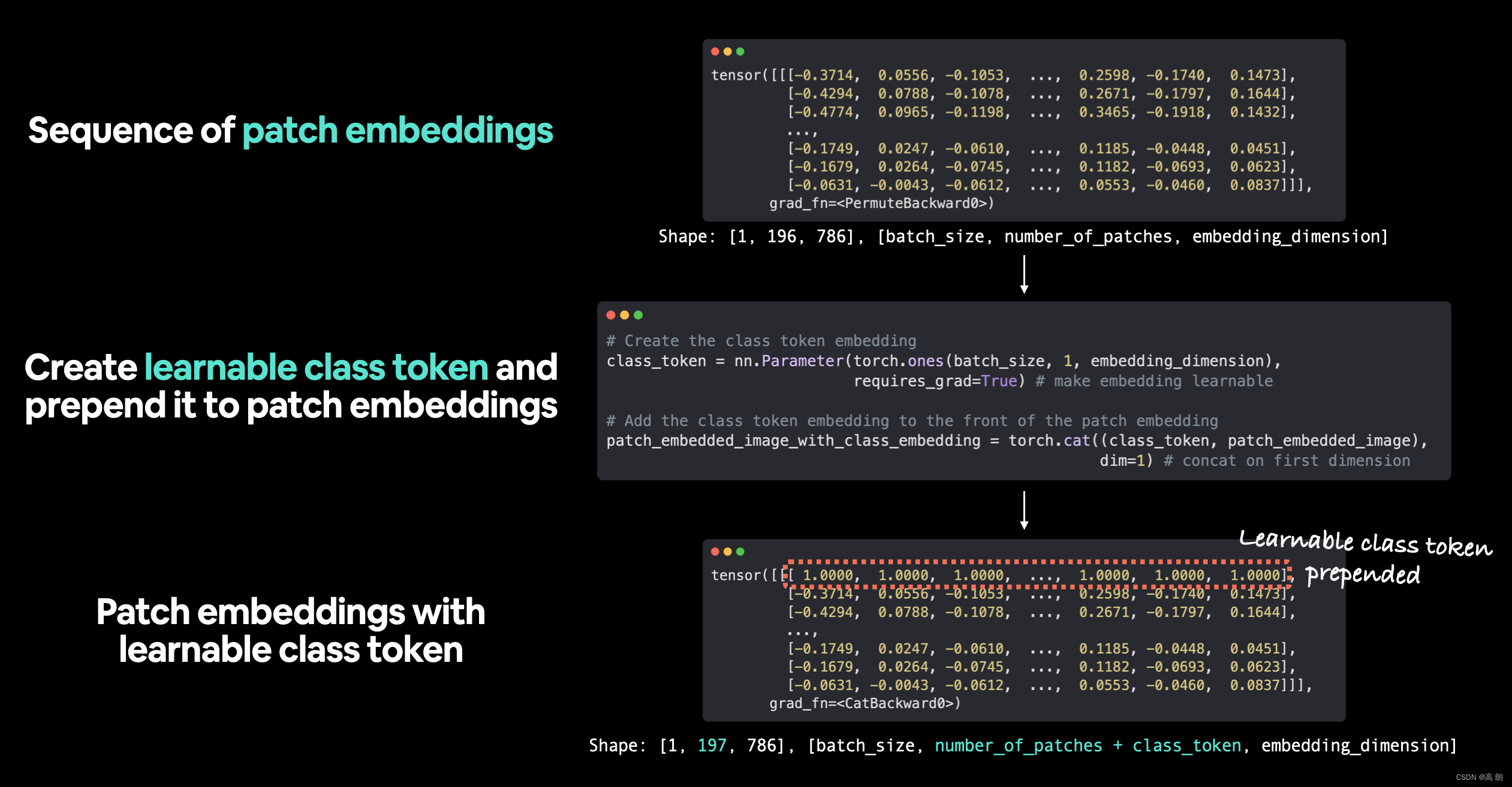
回顾:为创建可学习class token 所做的工作,我们从 PatchEmbedding() 在单个图像上创建的一系列图像 patch嵌 入开始,然后创建一个可学习 class token ,每个嵌入都有一个值尺寸,然后将其添加到patch嵌入的原始序列之前。注意:使用 torch.ones() 创建可学习class token 主要仅用于演示目的,实际上,可能会使用 torch.randn() 创建它。
- 创建位置嵌入
公式1 中 E p o s E_{pos} Epos
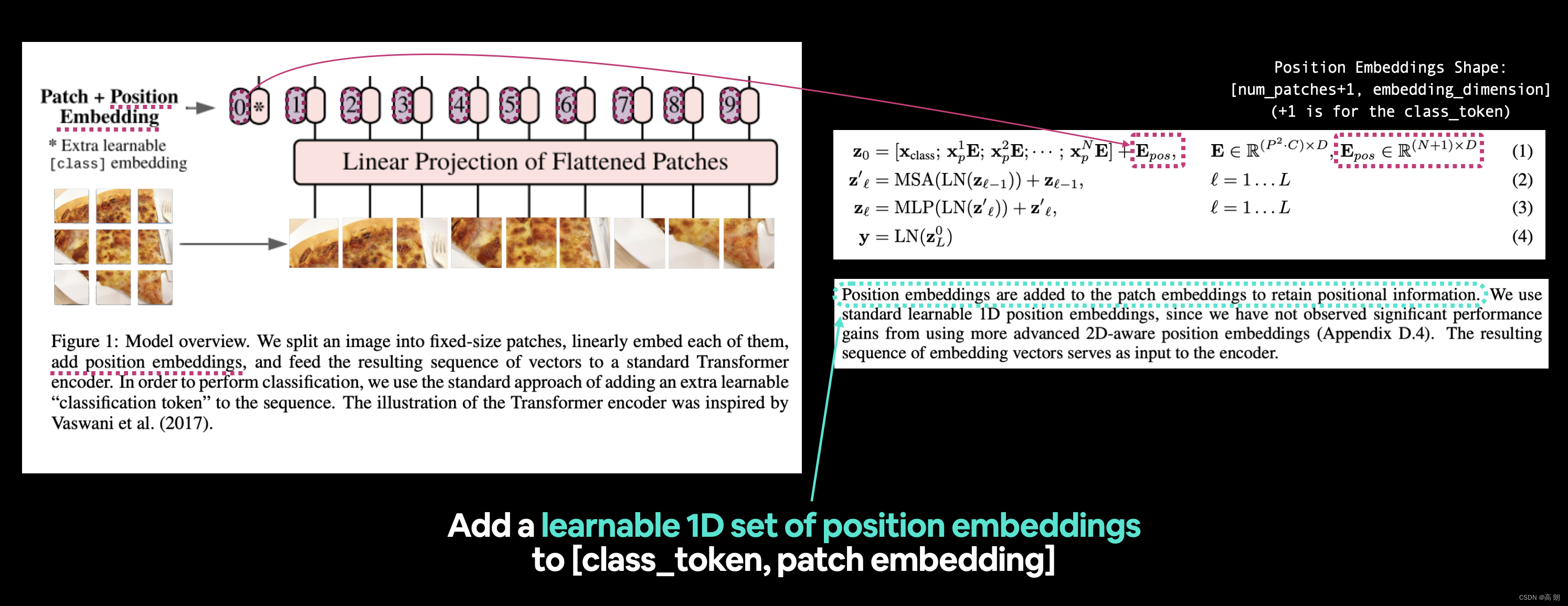 左:ViT 论文中的图 1,其中突出显示了我们要重新创建的位置嵌入。右:ViT 论文中与位置嵌入相关的公式 1 和第 3.1 节。
读 ViT 论文的第 3.1 节:
位置嵌入被添加到patch嵌入中以保留位置信息。我们使用标准的可学习 1D 位置嵌入,因为我们没有观察到使用更先进的 2D 感知位置嵌入带来的显着性能提升(附录 D.4)。生成的嵌入向量序列用作编码器的输入。
通过“保留位置信息”,作者的意思是他们希望架构知道patch的“顺序”。例如,patch二在patch一之后,patch三在patch二之后,依此类推。
在考虑图像中的内容时,此位置信息可能很重要(如果没有位置信息,则扁平序列可能会被视为没有顺序,因此没有 patch 与任何其他 patch 相关)。
开始创建位置嵌入,先查看当前的嵌入:
# View the sequence of patch embeddings with the prepended class embedding
patch_embedded_image_with_class_embedding, patch_embedded_image_with_class_embedding.shape
公式 1 指出位置嵌入 (
E
p
o
s
E_{pos}
Epos ) 的形状应为
(
D
+
1
)
×
N
(D+1) \times N
(D+1)×N
文中是:
E
pos
∈
R
(
N
+
1
)
×
D
E_{\text {pos }} \in R^{(N+1) \times D}
Epos ∈R(N+1)×D
- N = H W / P 2 N=HW/P^2 N=HW/P2 是生成的 patch 数量,它也充当 Transformer 的有效输入序列长度(patches 数量)。
- D 是 patch 嵌入的大小, D 的不同值可以在表 1(嵌入尺寸)中找到。
使用 torch.ones() 进行可学习的一维嵌入来创建 E p o s E_{pos} Epos:
# Calculate N (number of patches)
number_of_patches = int((height * width) / patch_size**2)

# Get embedding dimension
embedding_dimension = patch_embedded_image_with_class_embedding.shape[2]

# Create the learnable 1D position embedding
position_embedding = nn.Parameter(torch.ones(1,
                                             number_of_patches+1,
                                             embedding_dimension),
                                  requires_grad=True) # make sure it's learnable

# Show the first 10 sequences and 10 position embedding values and check the shape of the position embedding
print(position_embedding[:, :10, :10])
print(f"Position embeddding shape: {position_embedding.shape} -> [batch_size, number_of_patches, embedding_dimension]")
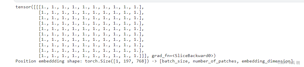
注意:仅出于演示目的将位置嵌入创建为 torch.ones() ,实际上, 可能会使用 torch.randn() 创建位置嵌入(从随机数开始并通过梯度下降进行改进) 。
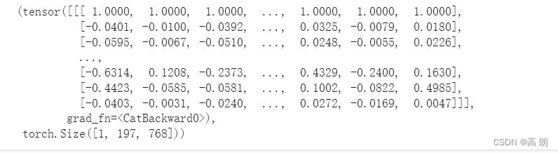
使用前置的 class token 将它们添加到 patch 嵌入序列中:
# Add the position embedding to the patch and class token embedding
patch_and_position_embedding = patch_embedded_image_with_class_embedding + position_embedding
print(patch_and_position_embedding)
print(f"Patch embeddings, class token prepended and positional embeddings added shape: {patch_and_position_embedding.shape} -> [batch_size, number_of_patches, embedding_dimension]")
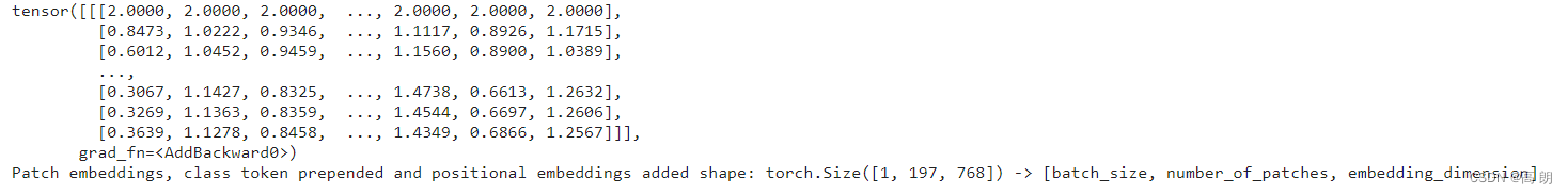 请注意嵌入张量中每个元素的值如何增加 1(这是因为使用 torch.ones() 创建位置嵌入)。
注意:如果愿意,可以将 class token 嵌入和位置嵌入放入它们自己的层中。稍后我们将在第 8 节中看到如何将它们合并到整个 ViT 架构的 forward() 方法中。
 我们用于将位置嵌入添加到 patch 嵌入和 class token 序列中的工作流程。注意: torch.ones() 仅用于出于说明目的创建嵌入,实际上,可能会使用 torch.randn() 以随机数开头。
- 将它们放在一起:从图像到嵌入
z 0 = [ x class ; x p 1 E ; x p 2 E ; ⋯ ; x p N E ] + E pos z_0=\left[x_{\text {class }} ; x_p^1 E ; x_p^2 E ; \cdots ; x_p^N E\right]+E_{\text {pos }} z0=[xclass ;xp1E;xp2E;⋯;xpNE]+Epos
E ∈ R ( P 2 ⋅ C ) × D , E pos ∈ R ( N + 1 ) × D E \in R^{\left(P^2 \cdot C\right) \times D}, E_{\text {pos }} \in R^{(N+1) \times D} E∈R(P2⋅C)×D,Epos ∈R(N+1)×D
开始将所有内容放在一个代码单元中,并从输入图像 ( x )到输出嵌入 ( z0 ):
(1)设置 patch 大小(我们将使用 16 ,因为它在整篇论文和 ViT-Base 中广泛使用)。
(2)获取单个图像,打印其形状并存储其高度和宽度。
(3)向单个图像添加批量维度,使其与我们的 PatchEmbedding 层兼容。
(4)使用 patch_size=16 和 embedding_dim=768 (来自 ViT-Base 的表 1)创建 PatchEmbedding 层。
(5)将单个图像传递到 4 中的 PatchEmbedding 层以创建 patch 嵌入序列。
(6)创建一个 class token 嵌入。
(7)将 class token 嵌入添加到步骤 5 中创建的 patch 嵌入之前。
(8)创建一个位置嵌入。
(9)将位置嵌入添加到步骤 7 中创建的 class token 和 patch 嵌入中。
还将确保使用 set_seeds() 设置随机种子,并一路打印出不同张量的形状:
set_seeds()
# 1. Set patch size
patch_size = 16
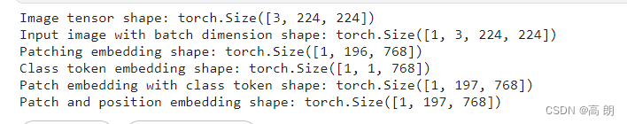
# 2. Print shape of original image tensor and get the image dimensions
print(f"Image tensor shape: {image.shape}")
height, width = image.shape[1], image.shape[2]
# 3. Get image tensor and add batch dimension
x = image.unsqueeze(0)
print(f"Input image with batch dimension shape: {x.shape}")
# 4. Create patch embedding layer
patch_embedding_layer = PatchEmbedding(in_channels=3,
patch_size=patch_size,
embedding_dim=768)
# 5. Pass image through patch embedding layer
patch_embedding = patch_embedding_layer(x)
print(f"Patching embedding shape: {patch_embedding.shape}")
# 6. Create class token embedding
batch_size = patch_embedding.shape[0]
embedding_dimension = patch_embedding.shape[-1]
class_token = nn.Parameter(torch.ones(batch_size, 1, embedding_dimension),
requires_grad=True) # make sure it's learnable
print(f"Class token embedding shape: {class_token.shape}")
# 7. Prepend class token embedding to patch embedding
patch_embedding_class_token = torch.cat((class_token, patch_embedding), dim=1)
print(f"Patch embedding with class token shape: {patch_embedding_class_token.shape}")
# 8. Create position embedding
number_of_patches = int((height * width) / patch_size**2)
position_embedding = nn.Parameter(torch.ones(1, number_of_patches+1, embedding_dimension),
requires_grad=True) # make sure it's learnable
# 9. Add position embedding to patch embedding with class token
patch_and_position_embedding = patch_embedding_class_token + position_embedding
print(f"Patch and position embedding shape: {patch_and_position_embedding.shape}")
 将 ViT 论文中的公式 1 映射到我们的 PyTorch 代码。这就是论文 复现的本质,将研究论文转化为可用的代码。
现在我们有了一种方法来对图像进行编码并将其传递给 ViT 论文图 1 中的 Transformer Encoder:

对整个 ViT 工作流程进行动画处理:从 patch 嵌入到transformer编码器再到 MLP 头。从代码的角度来看,创建 patch 嵌入可能是 复现 ViT 论文的最大部分。ViT 论文的许多其他部分(例如 Multi-Head Attention 和 Norm 层)可以使用现有的 PyTorch 层创建。
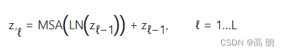
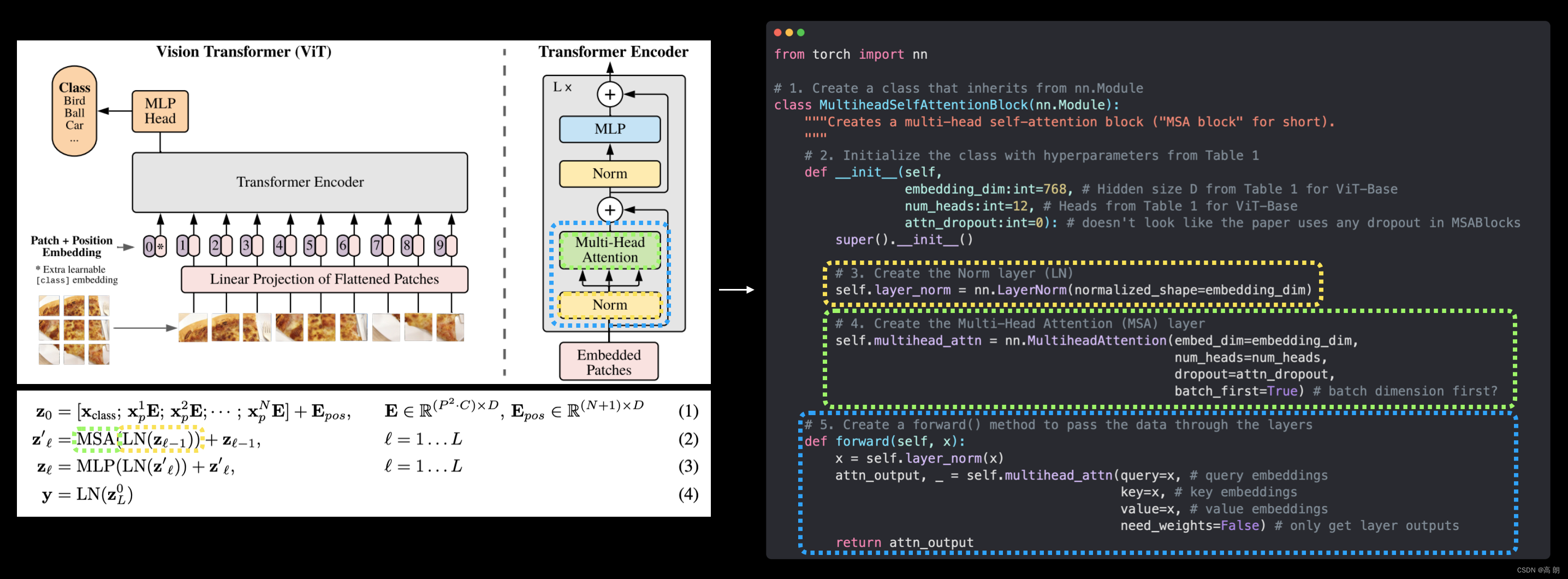
5. Equation 2: Multi-Head Attention (MSA)
多头注意力 (MSA)
将 Transformer Encoder 部分分为两部分(从小处开始,必要时增加):公式2 和 公式3。
z ℓ ′ = MSA ( LN ( z ℓ − 1 ) ) + z ℓ − 1 z_{\ell}^{\prime}=\operatorname{MSA}\left(\operatorname{LN}\left(z_{\ell-1}\right)\right) +z_{\ell-1} zℓ′=MSA(LN(zℓ−1))+zℓ−1
这表示多头注意力 (MSA) 层包裹在具有残差连接的 LayerNorm (LN) 层中(该层的输入被添加到该层的输出中)。
将公式 2 称为“MSA 块”。
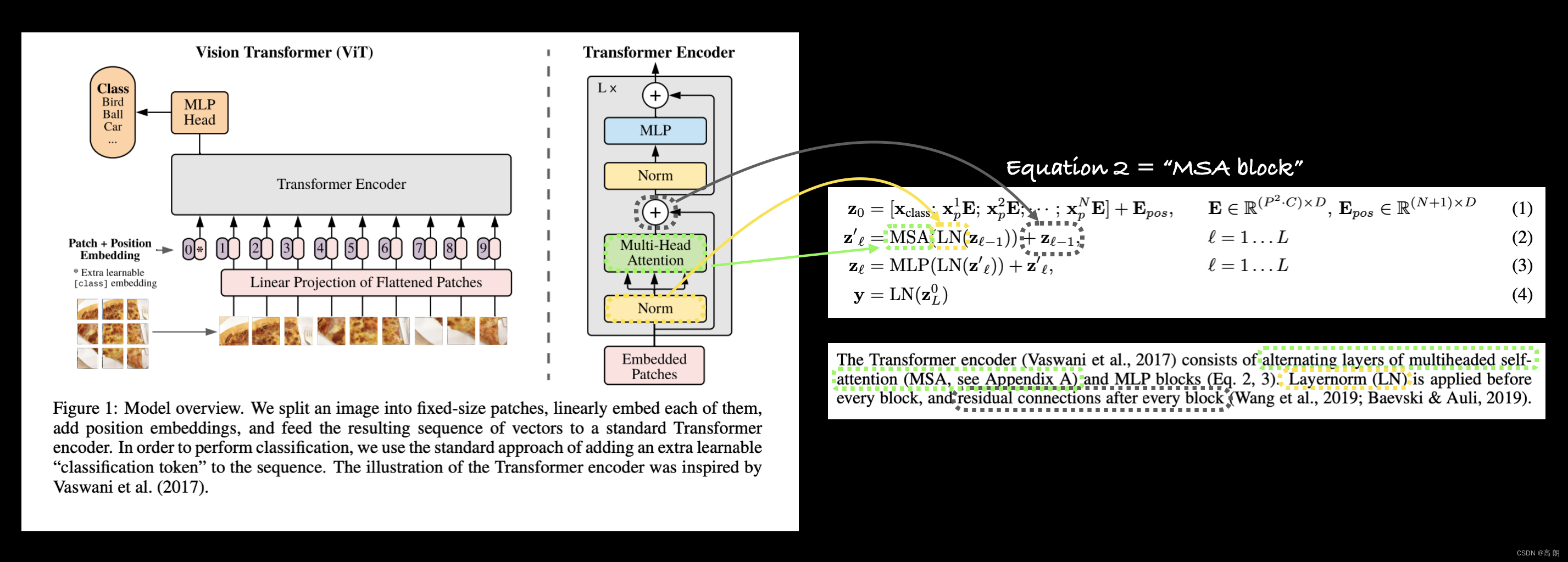
左: 图 1 来自 ViT 论文,其中包含多头注意力层和范数层,以及 Transformer Encoder 块中突出显示的残差连接 (+)。右图:将多头自注意力 (MSA) 层、规范层和残差连接映射到 ViT 论文中公式 2 的相应部分。
在研究论文中发现的许多层已经在 PyTorch 等现代深度学习框架中实现:
- Multi-Head Self Attention (MSA) -
torch.nn.MultiheadAttention(). - Norm(LN 或 LayerNorm)-
torch.nn.LayerNorm()。 - Residual connection:将输入添加到输出。
- LayerNorm(LN)层
层归一化( torch.nn.LayerNorm() 或 Norm 或 LayerNorm 或 LN)对最后一个维度上的输入进行归一化。
PyTorch 的 torch.nn.LayerNorm() 的主要参数是 normalized_shape 我们可以将其设置为等于我们想要标准化的维度大小(在我们的例子中它将是 D 或 768 对于 ViT-Base)。
层归一化有助于缩短训练时间和模型泛化(适应看不见的数据的能力)。
可以将任何类型的标准化视为“将数据转换为相似的格式”或“将数据样本转换为相似的分布”。神经网络可以比具有不同分布(相似的均值和标准差)的数据样本更容易地优化具有相似分布(相似的均值和标准差)的数据样本分布。
- The Multi-Head Self Attention (MSA) layer
多头自注意力(MSA)层
Attention is all you need 研究论文中介绍的原始 Transformer 架构以原始 Transformer 架构的形式揭示了自注意力和多头注意力(自注意力多次应用)的强大功能。
最初是为文本输入而设计的,原始的自注意力机制采用一系列单词,然后计算哪个单词应该更多地“关注”另一个单词。
换句话说,在“狗跳过栅栏”这句话中,也许“狗”这个词与“跳跃”和“栅栏”密切相关。
由于我们的输入是一系列图像块而不是单词,因此自注意力和多头注意力将计算图像的哪个块与另一个块最相关,最终形成图像的学习表示。
最重要的是,该层在给定数据的情况下自行完成此操作(我们不告诉它要学习哪些模式)。
使用 MSA 形成的层所学习的表示良好,我们将在模型的性能中看到结果。
Transformer 架构和注意力机制的更多信息:Illustlated Transformer 和 Illustratored Attention 。
将更多地关注对现有 PyTorch MSA 实现进行编码,而不是创建我们自己的实现,你可以发现 ViT 论文的 MSA 实现的正式定义在附录 A 中定义:
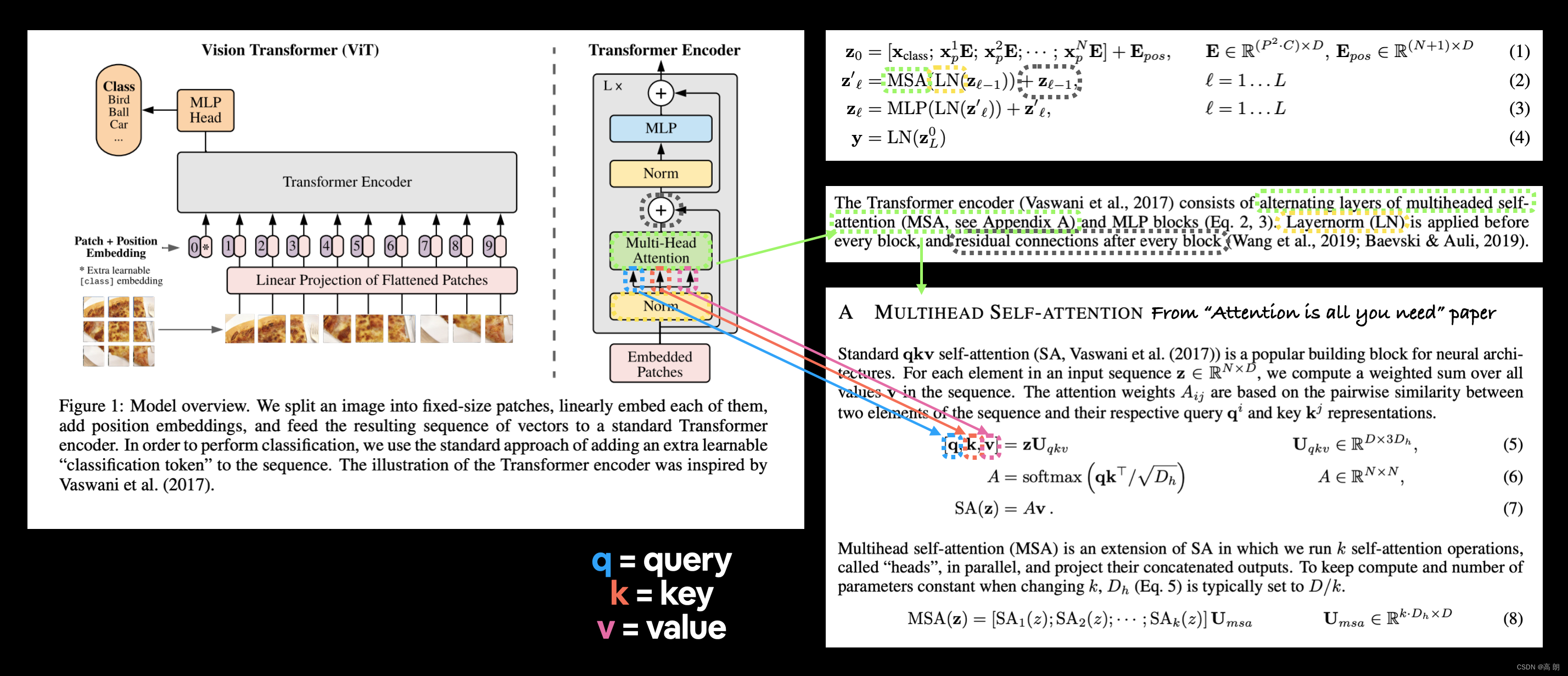 左: ViT 论文图 1 中的 Vision Transformer 架构概述。右图:ViT 论文的公式 2、第 3.1 节和附录 A 的定义在图 1 中突出显示,以反映其各自的部分。
上图突出显示了 MSA 层的三重嵌入输入,这被称为查询、键、值输入或简称为 qkv,它是自注意力机制的基础。在我们的例子中,三重嵌入输入将是 Norm 层输出的三个版本,一个用于查询、键和值。或者我们在前面创建的层归一化图像块和位置嵌入的三个版本。
可以使用 torch.nn.MultiheadAttention() 参数在 PyTorch 中实现 MSA 层:
embed_dim- 表 1 中的嵌入尺寸(隐藏尺寸 D)num_heads- 使用多少个注意力头(这就是术语“多头”的由来),这个值也在表 1(头)中。dropout- 是否对注意力层应用 dropout(根据附录 B.1,在 qkv-projections 之后不使用 dropout)。batch_first- 批量维度是第一位的。
- 使用 PyTorch 层复现公式 2
将公式 2 中关于 LayerNorm (LN) 和多头注意力 (MSA) 层讨论的所有内容付诸实践:
(1)创建一个名为 MultiheadSelfAttentionBlock 的类,该类继承自 torch.nn.Module 。
(2)使用 ViT 论文表 1 中的 ViT-Base 模型的超参数初始化该类。
(3)使用 torch.nn.LayerNorm() 创建一个层归一化 (LN) 层,其 normalized_shape 参数与我们的嵌入维度相同(表 1 中的 D )。
(4)使用适当的 embed_dim 、 num_heads 、 dropout 和 batch_first 参数创建多头注意力 (MSA) 层。
(5)为类创建一个 forward() 方法,通过 LN 层和 MSA 层传递输入。
# 1. Create a class that inherits from nn.Module
class MultiheadSelfAttentionBlock(nn.Module):
    """Creates a multi-head self-attention block ("MSA block" for short).
    """
    # 2. Initialize the class with hyperparameters from Table 1
    def __init__(self,
                 embedding_dim:int=768, # Hidden size D from Table 1 for ViT-Base
                 num_heads:int=12, # Heads from Table 1 for ViT-Base
                 attn_dropout:float=0): # doesn't look like the paper uses any dropout in MSABlocks
        super().__init__()

        # 3. Create the Norm layer (LN)
        self.layer_norm = nn.LayerNorm(normalized_shape=embedding_dim)

        # 4. Create the Multi-Head Attention (MSA) layer
        self.multihead_attn = nn.MultiheadAttention(embed_dim=embedding_dim,
                                                    num_heads=num_heads,
                                                    dropout=attn_dropout,
                                                    batch_first=True) # does our batch dimension come first?

    # 5. Create a forward() method to pass the data throguh the layers
    def forward(self, x):
        x = self.layer_norm(x)
        attn_output, _ = self.multihead_attn(query=x, # query embeddings
                                             key=x, # key embeddings
                                             value=x, # value embeddings
                                             need_weights=False) # do we need the weights or just the layer outputs?
        return attn_output
注意:与图 1 不同,我们的 MultiheadSelfAttentionBlock 不包含跳过或剩余连接(公式 2 中的“ + z ℓ − 1 +z_{ℓ−1} +zℓ−1”),后续将包含此连接在 7.1 节中创建整个 Transformer Encoder 时。
通过创建 MultiheadSelfAttentionBlock 的实例并传递到前面创建的 patch_and_position_embedding 变量来尝试一下
# Create an instance of MSABlock
multihead_self_attention_block = MultiheadSelfAttentionBlock(embedding_dim=768, # from Table 1
                                                             num_heads=12) # from Table 1

# Pass patch and position image embedding through MSABlock
patched_image_through_msa_block = multihead_self_attention_block(patch_and_position_embedding)
print(f"Input shape of MSA block: {patch_and_position_embedding.shape}")
print(f"Output shape MSA block: {patched_image_through_msa_block.shape}")
Input shape of MSA block: torch.Size([1, 197, 768])
Output shape MSA block: torch.Size([1, 197, 768])
当数据通过 MSA 块时,数据的输入和输出形状如何保持不变。这并不意味着数据在变化过程中不会发生变化。可以尝试打印输入和输出张量以查看它如何变化(尽管这种变化将跨越 1 * 197 * 768 值并且可能很难可视化)。
 左: 图 1 中的 Vision Transformer 架构,突出显示了多头注意力层和 LayerNorm 层,这些层构成了论文第 3.1 节中的公式 2。右图:使用 PyTorch 层 复现公式 2(末尾没有跳跃连接)。
现在已经正式复现了公式 2(除了最后的残差连接,我们将在 7. 节中讨论这一点)
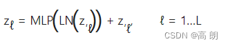
6. Equation 3: Multilayer Perceptron (MLP)
MLP 代表“多层感知器”,LN 代表“层归一化”,最后添加的是skip/residual连接。
将公式 3 称为 Transformer 编码器的“MLP 块”(注意我们如何继续将架构分解为更小的块的趋势)。
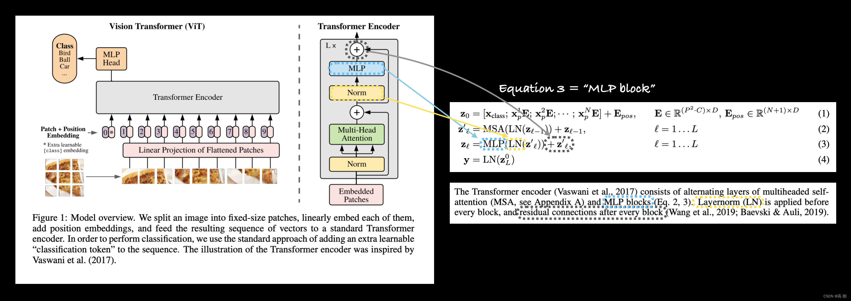 左: ViT 论文中的图 1,其中包含 MLP 和 Norm 层以及 Transformer Encoder 块中突出显示的残差连接 (+)。右图:将多层感知器 (MLP) 层、规范层 (LN) 和残差连接映射到 ViT 论文中公式 3 的相应部分。
- The MLP layer(s)
MLP 一词非常广泛,因为它几乎可以指多层的任何组合(因此多层感知器中的“多”),linear layer -> non-linear layer -> linear layer -> non-linear layer。
以 ViT 论文为例,MLP 结构在第 3.1 节中定义:MLP 包含两个具有 GELU 非线性的层。
其中“两层”是指线性层(PyTorch 中的 torch.nn.Linear() ),“GELU 非线性”是 GELU(高斯误差线性单位)非线性激活函数(PyTorch 中的 torch.nn.GELU() 火炬)。
注意:线性层(
torch.nn.Linear())有时也可以称为“密集层”或“前馈层”。有些论文甚至使用所有三个术语来描述同一事物(如 ViT 论文中所示)。
关于 MLP 块的另一个偷偷摸摸的细节直到附录 B.1(训练)才出现:表 3 总结了我们针对不同模型的训练设置。 …使用时,Dropout 应用于除 qkv 投影之外的每个密集层之后,以及直接在添加位置到 patch 嵌入之后应用。
这意味着 MLP 块中的每个线性层都有一个 dropout 层(PyTorch 中的 torch.nn.Dropout() )。
其值可以在ViT论文的表3中找到(对于ViT-Base, dropout=0.1 )。
MLP 块的结构将是:layer norm -> linear layer -> non-linear layer -> dropout -> linear layer -> dropout
表 1 中提供了线性层的超参数值(MLP 大小是线性层之间隐藏单元的数量,隐藏大小 D 是 MLP 块的输出大小) 。
- 使用 PyTorch 层复现公式 3
将公式 3 中的 LayerNorm (LN) 和 MLP (MSA) 层所讨论的所有内容付诸实践:
(1)创建一个名为 MLPBlock 的类,该类继承自 torch.nn.Module 。
(2)使用 ViT-Base 模型的 ViT 论文表 1 和表 3 中的超参数初始化该类。
(3)使用 torch.nn.LayerNorm() 创建一个层归一化 (LN) 层,其 normalized_shape 参数与我们的嵌入维度相同(表 1 中的 D )。
(4)使用 torch.nn.Linear() 、 torch.nn.Dropout() 和 torch.nn.GELU() 以及表 1 和表 3 中适当的超参数值创建一系列连续的 MLP 层。
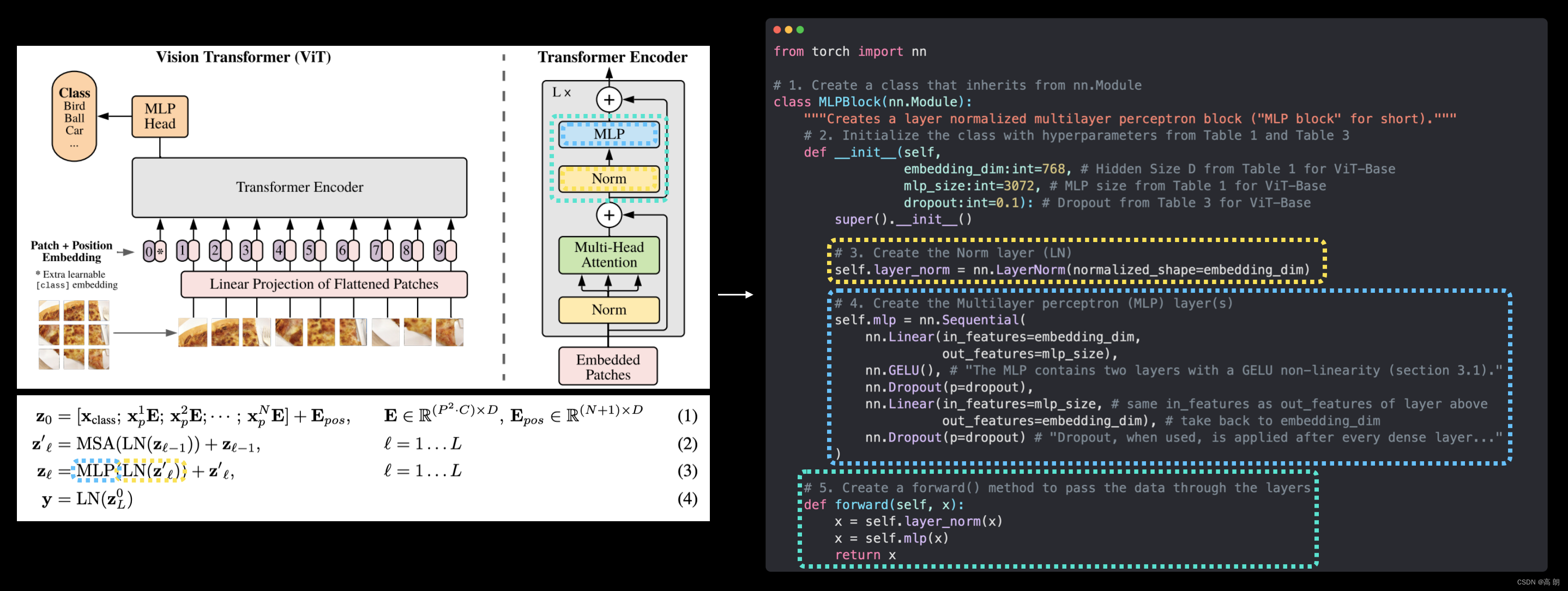
(5)为类创建一个 forward() 方法,通过 LN 层和 MLP 层传递输入。
# 1. Create a class that inherits from nn.Module
class MLPBlock(nn.Module):
    """Creates a layer normalized multilayer perceptron block ("MLP block" for short)."""
    # 2. Initialize the class with hyperparameters from Table 1 and Table 3
    def __init__(self,
                 embedding_dim:int=768, # Hidden Size D from Table 1 for ViT-Base
                 mlp_size:int=3072, # MLP size from Table 1 for ViT-Base
                 dropout:float=0.1): # Dropout from Table 3 for ViT-Base
        super().__init__()

        # 3. Create the Norm layer (LN)
        self.layer_norm = nn.LayerNorm(normalized_shape=embedding_dim)

        # 4. Create the Multilayer perceptron (MLP) layer(s)
        self.mlp = nn.Sequential(
            nn.Linear(in_features=embedding_dim,
                      out_features=mlp_size),
            nn.GELU(), # "The MLP contains two layers with a GELU non-linearity (section 3.1)."
            nn.Dropout(p=dropout),
            nn.Linear(in_features=mlp_size, # needs to take same in_features as out_features of layer above
                      out_features=embedding_dim), # take back to embedding_dim
            nn.Dropout(p=dropout) # "Dropout, when used, is applied after every dense layer.."
        )

    # 5. Create a forward() method to pass the data throguh the layers
    def forward(self, x):
        x = self.layer_norm(x)
        x = self.mlp(x)
        return x
注意:与图 1 不同,我们的 MLPBlock() 不包含跳过或剩余连接(公式 3 中的“ + z ℓ ′ +z^′_ℓ +zℓ′ ”),我们将包含此连接当我们稍后创建整个 Transformer 编码器时。
通过创建 MLPBlock 的实例并传递到前面创建的 patched_image_through_msa_block 变量来测试一下:
# Create an instance of MLPBlock
mlp_block = MLPBlock(embedding_dim=768, # from Table 1
                     mlp_size=3072, # from Table 1
                     dropout=0.1) # from Table 3

# Pass output of MSABlock through MLPBlock
patched_image_through_mlp_block = mlp_block(patched_image_through_msa_block)
print(f"Input shape of MLP block: {patched_image_through_msa_block.shape}")
print(f"Output shape MLP block: {patched_image_through_mlp_block.shape}")
Input shape of MLP block: torch.Size([1, 197, 768])
Output shape MLP block: torch.Size([1, 197, 768])
请注意,当数据进入和离开 MLP 模块时,数据的输入和输出形状如何再次保持相同。然而,当数据通过 MLP 块内的 nn.Linear() 层时,形状确实会发生变化(从表 1 扩展到 MLP 大小,然后压缩回隐藏大小 D(来自表 1)。
 左图:图 1 中的 Vision Transformer 架构,其中突出显示了 MLP 和 Norm 层,这些层构成了论文第 3.1 节中的公式 3。右图:使用 PyTorch 层 复现公式 3(末尾没有跳跃连接)。
复现公式 3(除了最后的剩余连接,我们将在第 7. 节中讨论这一点)!
已经在 PyTorch 代码中得到了公式 2 和 3,现在让我们将它们放在一起来创建 Transformer 编码器。
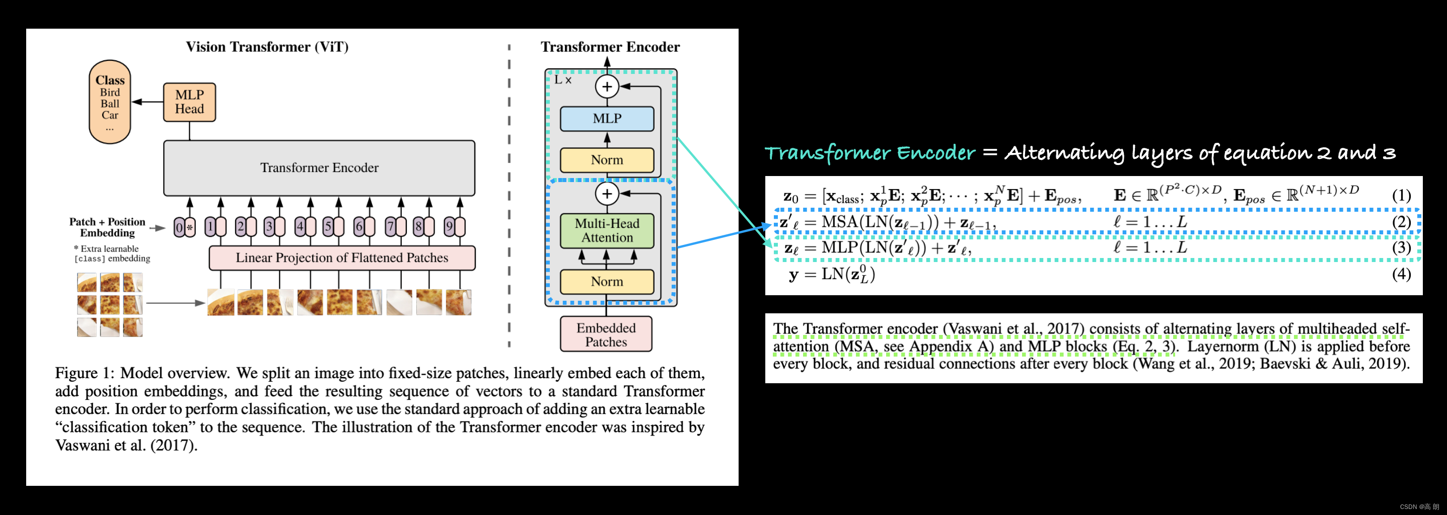
7. 创建 Transformer 编码器
将 MultiheadSelfAttentionBlock (公式 2)和 MLPBlock (公式 3)堆叠在一起并创建 ViT 架构的 Transformer 编码器了。
在深度学习中,“编码器”或“自动编码器”通常指的是对输入进行“编码”(将其转换为某种形式的数字表示)的一层堆栈。
Transformer 编码器将使用一系列 MSA 块和 MLP 块的交替层将我们的修补图像嵌入编码为学习表示,如 ViT 论文第 3.1 节所述:
Transformer 编码器(Vaswani 等人,2017)由多头自注意力(MSA,参见附录 A)和 MLP 块(公式 2、3)的交替层组成。 Layernorm (LN) 应用在每个块之前,并在每个块之后应用残差连接(Wang et al., 2019;Baevski & Auli, 2019)。
已经创建了 MSA 和 MLP 块,剩余连接-残差连接(也称为跳跃连接)首先在论文“图像识别的深度残差学习”中引入,并通过在其后续输出中添加层输入来实现。子序列输出可能是一层或多层之后的。在 ViT 架构的情况下,残余连接意味着 MSA 块的输入在传递到 MLP 块之前被添加回 MSA 块的输出。在 MLP 块进入下一个 Transformer Encoder 块之前,也会发生同样的事情。
x_input -> MSA_block -> [MSA_block_output + x_input] -> MLP_block -> [MLP_block_output + MSA_block_output + x_input] -> ...
残差连接背后的主要思想之一是它们防止权重值和梯度更新变得太小,从而允许更深的网络,进而允许学习更深的表示。
注:标志性的计算机视觉架构“ResNet”因引入残差连接而得名。 可以在 torchvision.models 中找到许多 ResNet 架构的预训练版本。
- 通过组合我们定制的层来创建 Transformer Encoder
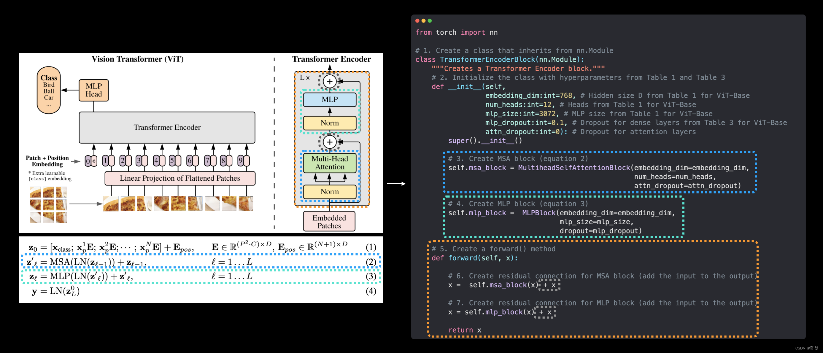
开始使用 PyTorch 制作 ViT Transformer 编码器:
(1)创建一个名为TransformerEncoderBlock的类,该类继承自torch.nn.Module。
(2)使用 ViT-Base 模型的 ViT 论文表 1 和表 3 中的超参数初始化该类。
(3)使用第 5. 节中的 MultiheadSelfAttentionBlock 和适当的参数实例化公式 2 的 MSA 块。
(4)使用第 6. 节中的 MLPBlock 和适当的参数实例化公式 3 的 MLP 块。
(5)为我们的 TransformerEncoderBlock 类创建一个 forward() 方法。
(6)为 MSA 模块创建残差连接(对于公式 2)。
(7)为 MLP 模块创建残差连接(对于公式 3)。
# 1. Create a class that inherits from nn.Module
class TransformerEncoderBlock(nn.Module):
    """Creates a Transformer Encoder block."""
    # 2. Initialize the class with hyperparameters from Table 1 and Table 3
    def __init__(self,
                 embedding_dim:int=768, # Hidden size D from Table 1 for ViT-Base
                 num_heads:int=12, # Heads from Table 1 for ViT-Base
                 mlp_size:int=3072, # MLP size from Table 1 for ViT-Base
                 mlp_dropout:float=0.1, # Amount of dropout for dense layers from Table 3 for ViT-Base
                 attn_dropout:float=0): # Amount of dropout for attention layers
        super().__init__()

        # 3. Create MSA block (equation 2)
        self.msa_block = MultiheadSelfAttentionBlock(embedding_dim=embedding_dim,
                                                     num_heads=num_heads,
                                                     attn_dropout=attn_dropout)

        # 4. Create MLP block (equation 3)
        self.mlp_block =  MLPBlock(embedding_dim=embedding_dim,
                                   mlp_size=mlp_size,
                                   dropout=mlp_dropout)

    # 5. Create a forward() method
    def forward(self, x):

        # 6. Create residual connection for MSA block (add the input to the output)
        x =  self.msa_block(x) + x

        # 7. Create residual connection for MLP block (add the input to the output)
        x = self.mlp_block(x) + x

        return x
 左: ViT 论文中的图 1,突出显示了 ViT 架构的 Transformer Encoder。右:Transformer 编码器映射到 ViT 论文的公式 2 和 3,Transformer 编码器由公式 2(多头注意力)和公式 3(多层感知器)的交替块组成。
将 ViT Transformer Encoder 映射到代码:
 ViT 论文中的表 1 有一个“层”列。这是指特定 ViT 架构中 Transformer Encoder 块的数量。我们将把 12 个 Transformer Encoder 块堆叠在一起,以形成我们架构的主干(在第 8. 节中介绍这一点)。
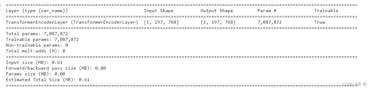
用 torchinfo.summary() ,将形状 (1, 197, 768) -> (batch_size, num_patches, embedding_dimension) 的输入传递给我们的 Transformer Encoder 块:
# Create an instance of TransformerEncoderBlock
transformer_encoder_block = TransformerEncoderBlock()

# # Print an input and output summary of our Transformer Encoder (uncomment for full output)
summary(model=transformer_encoder_block,
        input_size=(1, 197, 768), # (batch_size, num_patches, embedding_dimension)
        col_names=["input_size", "output_size", "num_params", "trainable"],
        col_width=20,
        row_settings=["var_names"])
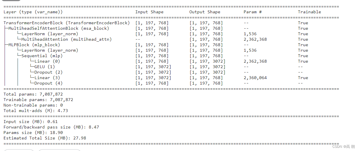 可以看到输入在 Transformer Encoder 块的 MSA 块和 MLP 块中的所有各个层中移动时形状发生变化,最后最终返回到其原始形状。
注意:仅仅因为 Transformer Encoder 块的输入在块的输出处具有相同的形状并不意味着这些值没有被操纵,Transformer Encoder 块(并将它们堆叠在一起)的整个目标是学习使用中间的各个层对输入进行深度表示。
- 使用 PyTorch 的 Transformer 层创建 Transformer 编码器
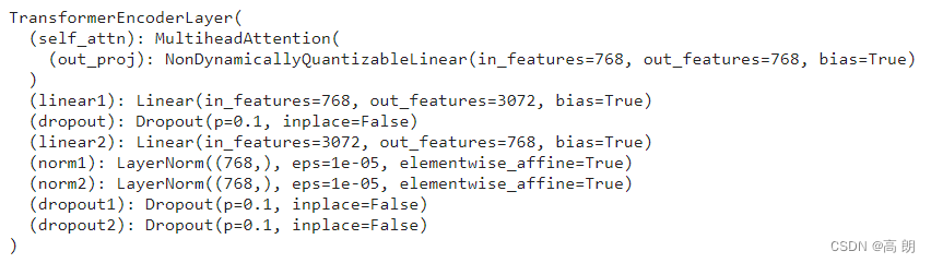
已经自己构建了 Transformer Encoder 层的组件和层本身,但由于其受欢迎程度和有效性的提高,PyTorch 现在拥有内置 Transformer 层作为 torch.nn 的一部分。可以使用torch.nn.TransformerEncoderLayer()重新创建刚刚创建的 TransformerEncoderBlock 并设置与上面相同的超参数。
# Create the same as above with torch.nn.TransformerEncoderLayer()
torch_transformer_encoder_layer = nn.TransformerEncoderLayer(d_model=768, # Hidden size D from Table 1 for ViT-Base
                                                             nhead=12, # Heads from Table 1 for ViT-Base
                                                             dim_feedforward=3072, # MLP size from Table 1 for ViT-Base
                                                             dropout=0.1, # Amount of dropout for dense layers from Table 3 for ViT-Base
                                                             activation="gelu", # GELU non-linear activation
                                                             batch_first=True, # Do our batches come first?
                                                             norm_first=True) # Normalize first or after MSA/MLP layers?

torch_transformer_encoder_layer
 用 torchinfo.summary() 得到该模型摘要:
# # Get the output of PyTorch's version of the Transformer Encoder (uncomment for full output)
summary(model=torch_transformer_encoder_layer,
        input_size=(1, 197, 768), # (batch_size, num_patches, embedding_dimension)
        col_names=["input_size", "output_size", "num_params", "trainable"],
        col_width=20,
        row_settings=["var_names"])
由于 torch.nn.TransformerEncoderLayer() 构建其层的方式,摘要的输出与我们的略有不同,但它使用的层、参数数量以及输入和输出形状是相同的。
最后,由于 ViT 架构使用多个 Transformer 层,每个层堆叠在整个架构的顶部(表 1 显示 ViT-Base 的情况下有 12 层),因此 可以使用 torch.nn.TransformerEncoder(encoder_layer, num_layers) 执行此操作,其中:
encoder_layer- 使用 torch.nn.TransformerEncoderLayer() 创建的目标 Transformer Encoder 层。num_layers- 要堆叠在一起的 Transformer Encoder 层的数量。
8. 将它们放在一起创建 ViT
从 patch 和位置嵌入到 Transformer 编码器再到 MLP Head,最后还剩公式4:
y
=
L
N
(
z
L
0
)
y = LN(z^0_L)
y=LN(zL0)
只是一个 torch.nn.LayerNorm() 层和一个 torch.nn.Linear() 层来转换 Transformer Encoder logit 输出的第 0 个索引 (
z
L
0
z^0_L
zL0)达到我们的目标class数量。
要创建完整的架构,我们还需要将许多 TransformerEncoderBlock 堆叠在一起,我们可以通过将它们的列表传递给 torch.nn.Sequential() 来做到这一点(这将形成一个 TransformerEncoderBlock 的连续范围)。
重点关注表 1 中的 ViT-Base 超参数,但代码应该适用于其他 ViT 变体:
(1)创建一个名为 ViT 的类,该类继承自 torch.nn.Module 。
(2)使用 ViT-Base 模型的 ViT 论文表 1 和表 3 中的超参数初始化该类。
(3)确保图像大小可以被 patch 大小整除(图像应该被分割成均匀的 patch )。
(4)使用公式
N
=
H
W
/
P
2
N=HW/P^2
N=HW/P2 计算 patch 数量,其中 H 是图像高度, W 是图像宽度, P 是 patch 大小。
(5)创建一个可学习的class 嵌入 token(公式 1),如上面第 4. 节中所做的那样。
(6)创建一个可学习的位置嵌入向量(公式 1),如上面第 4. 节中所做的那样。
(7)按照 ViT 论文附录 B.1 中的讨论设置嵌入 dropout 层。
(8)使用 4. 节中的 PatchEmbedding 类创建 patch 嵌入层。
(9)通过将第 7. 节中创建的 TransformerEncoderBlock 列表传递到 torch.nn.Sequential() (公式 2 和 3)来创建一系列 Transformer Encoder 块。
(10)通过传递 torch.nn.LayerNorm() (LN) 层和 torch.nn.Linear(out_features=num_classes) 层(其中 num_classes 是目标数)来创建 MLP 头(也称为分类器头或公式 4)类)线性层到 torch.nn.Sequential() 。
(11)创建一个接受输入的 forward() 方法。
(12)获取输入的批量大小(形状的第一个维度)。
(13)使用步骤 8 中创建的层(公式 1)创建修补嵌入。
(14)使用步骤 5 中创建的层创建 class token 嵌入,并使用 torch.Tensor.expand() (公式 1)将其扩展到步骤 11 中找到的批次数量。
(15)使用 torch.cat() (公式 1)将步骤 13 中创建的 class token 嵌入连接到步骤 12 中创建的 patch 嵌入的第一个维度。
(16)将步骤 6 中创建的位置嵌入添加到步骤 14 中创建的 patch 和 class token 嵌入(公式 1)。
(17)将 patch 和位置嵌入传递到步骤 7 中创建的 dropout 层。
(18)将步骤 16 中的 patch 和位置嵌入传递到步骤 9 中创建的 Transformer Encoder 层堆栈(公式 2 和 3)。
(19)将步骤 17 中的 Transformer Encoder 层堆栈的输出的索引 0 传递到步骤 10 中创建的分类器头(公式 4)。
(20)构建完成,Vision Transformer
# 1. Create a ViT class that inherits from nn.Module
class ViT(nn.Module):
    """Creates a Vision Transformer architecture with ViT-Base hyperparameters by default."""
    # 2. Initialize the class with hyperparameters from Table 1 and Table 3
    def __init__(self,
                 img_size:int=224, # Training resolution from Table 3 in ViT paper
                 in_channels:int=3, # Number of channels in input image
                 patch_size:int=16, # Patch size
                 num_transformer_layers:int=12, # Layers from Table 1 for ViT-Base
                 embedding_dim:int=768, # Hidden size D from Table 1 for ViT-Base
                 mlp_size:int=3072, # MLP size from Table 1 for ViT-Base
                 num_heads:int=12, # Heads from Table 1 for ViT-Base
                 attn_dropout:float=0, # Dropout for attention projection
                 mlp_dropout:float=0.1, # Dropout for dense/MLP layers
                 embedding_dropout:float=0.1, # Dropout for patch and position embeddings
                 num_classes:int=1000): # Default for ImageNet but can customize this
        super().__init__() # don't forget the super().__init__()!

        # 3. Make the image size is divisble by the patch size
        assert img_size % patch_size == 0, f"Image size must be divisible by patch size, image size: {img_size}, patch size: {patch_size}."

        # 4. Calculate number of patches (height * width/patch^2)
        self.num_patches = (img_size * img_size) // patch_size**2

        # 5. Create learnable class embedding (needs to go at front of sequence of patch embeddings)
        self.class_embedding = nn.Parameter(data=torch.randn(1, 1, embedding_dim),
                                            requires_grad=True)

        # 6. Create learnable position embedding
        self.position_embedding = nn.Parameter(data=torch.randn(1, self.num_patches+1, embedding_dim),
                                               requires_grad=True)

        # 7. Create embedding dropout value
        self.embedding_dropout = nn.Dropout(p=embedding_dropout)

        # 8. Create patch embedding layer
        self.patch_embedding = PatchEmbedding(in_channels=in_channels,
                                              patch_size=patch_size,
                                              embedding_dim=embedding_dim)

        # 9. Create Transformer Encoder blocks (we can stack Transformer Encoder blocks using nn.Sequential())
        # Note: The "*" means "all"
        self.transformer_encoder = nn.Sequential(*[TransformerEncoderBlock(embedding_dim=embedding_dim,
                                                                            num_heads=num_heads,
                                                                            mlp_size=mlp_size,
                                                                            mlp_dropout=mlp_dropout) for _ in range(num_transformer_layers)])

        # 10. Create classifier head
        self.classifier = nn.Sequential(
            nn.LayerNorm(normalized_shape=embedding_dim),
            nn.Linear(in_features=embedding_dim,
                      out_features=num_classes)
        )

    # 11. Create a forward() method
    def forward(self, x):

        # 12. Get batch size
        batch_size = x.shape[0]

        # 13. Create class token embedding and expand it to match the batch size (equation 1)
        class_token = self.class_embedding.expand(batch_size, -1, -1) # "-1" means to infer the dimension (try this line on its own)

        # 14. Create patch embedding (equation 1)
        x = self.patch_embedding(x)

        # 15. Concat class embedding and patch embedding (equation 1)
        x = torch.cat((class_token, x), dim=1)

        # 16. Add position embedding to patch embedding (equation 1)
        x = self.position_embedding + x

        # 17. Run embedding dropout (Appendix B.1)
        x = self.embedding_dropout(x)

        # 18. Pass patch, position and class embedding through transformer encoder layers (equations 2 & 3)
        x = self.transformer_encoder(x)

        # 19. Put 0 index logit through classifier (equation 4)
        x = self.classifier(x[:, 0]) # run on each sample in a batch at 0 index

        return x
创建一个快速演示来展示class token 嵌入在批量维度上扩展时发生的情况:
# Example of creating the class embedding and expanding over a batch dimension
batch_size = 32
class_token_embedding_single = nn.Parameter(data=torch.randn(1, 1, 768)) # create a single learnable class token
class_token_embedding_expanded = class_token_embedding_single.expand(batch_size, -1, -1) # expand the single learnable class token across the batch dimension, "-1" means to "infer the dimension"

# Print out the change in shapes
print(f"Shape of class token embedding single: {class_token_embedding_single.shape}")
print(f"Shape of class token embedding expanded: {class_token_embedding_expanded.shape}")
Shape of class token embedding single: torch.Size([1, 1, 768])
Shape of class token embedding expanded: torch.Size([32, 1, 768])
请注意第一个维度如何扩展到批量大小,而其他维度保持不变(因为它们是由 .expand(batch_size, -1, -1) 中的“ -1 ”维度推断出来的)。
测试 ViT() 类:
set_seeds()

# Create a random tensor with same shape as a single image
random_image_tensor = torch.randn(1, 3, 224, 224) # (batch_size, color_channels, height, width)

# Create an instance of ViT with the number of classes we're working with (pizza, steak, sushi)
vit = ViT(num_classes=len(class_names))

# Pass the random image tensor to our ViT instance
vit(random_image_tensor)
tensor([[-0.2377, 0.7360, 1.2137]], grad_fn=<AddmmBackward0>)
看起来我们的随机图像张量一直通过我们的 ViT 架构,并且输出三个 logit 值(每个类一个)。因为我们的 ViT 类有很多参数,所以如果我们愿意的话,我们可以自定义 img_size 、 patch_size 或 num_classes 。
- 获得 ViT 模型的直观总结
注意:ViT 论文指出使用 4096 的批量大小进行训练,但是,这需要大量的 CPU/GPU 计算内存来处理(批量大小越大,需要的内存就越多)。因此,为了确保不会出现内存错误,我们将坚持使用 32 的批处理大小。如果 可以访问具有更多内存的硬件, 可以随时增加此值。
from torchinfo import summary

# # Print a summary of our custom ViT model using torchinfo (uncomment for actual output)
summary(model=vit,
        input_size=(32, 3, 224, 224), # (batch_size, color_channels, height, width)
        # col_names=["input_size"], # uncomment for smaller output
        col_names=["input_size", "output_size", "num_params", "trainable"],
        col_width=20,
        row_settings=["var_names"]
)
============================================================================================================================================
Layer (type (var_name))                                      Input Shape          Output Shape         Param #              Trainable
============================================================================================================================================
ViT (ViT)                                                    [32, 3, 224, 224]    [32, 3]              152,064              True
├─PatchEmbedding (patch_embedding)                           [32, 3, 224, 224]    [32, 196, 768]       --                   True
│    └─Conv2d (patcher)                                      [32, 3, 224, 224]    [32, 768, 14, 14]    590,592              True
│    └─Flatten (flatten)                                     [32, 768, 14, 14]    [32, 768, 196]       --                   --
├─Dropout (embedding_dropout)                                [32, 197, 768]       [32, 197, 768]       --                   --
├─Sequential (transformer_encoder)                           [32, 197, 768]       [32, 197, 768]       --                   True
│    └─TransformerEncoderBlock (0)                           [32, 197, 768]       [32, 197, 768]       --                   True
│    │    └─MultiheadSelfAttentionBlock (msa_block)          [32, 197, 768]       [32, 197, 768]       2,363,904            True
│    │    └─MLPBlock (mlp_block)                             [32, 197, 768]       [32, 197, 768]       4,723,968            True
│    └─TransformerEncoderBlock (1)                           [32, 197, 768]       [32, 197, 768]       --                   True
│    │    └─MultiheadSelfAttentionBlock (msa_block)          [32, 197, 768]       [32, 197, 768]       2,363,904            True
│    │    └─MLPBlock (mlp_block)                             [32, 197, 768]       [32, 197, 768]       4,723,968            True
│    └─TransformerEncoderBlock (2)                           [32, 197, 768]       [32, 197, 768]       --                   True
│    │    └─MultiheadSelfAttentionBlock (msa_block)          [32, 197, 768]       [32, 197, 768]       2,363,904            True
│    │    └─MLPBlock (mlp_block)                             [32, 197, 768]       [32, 197, 768]       4,723,968            True
│    └─TransformerEncoderBlock (3)                           [32, 197, 768]       [32, 197, 768]       --                   True
│    │    └─MultiheadSelfAttentionBlock (msa_block)          [32, 197, 768]       [32, 197, 768]       2,363,904            True
│    │    └─MLPBlock (mlp_block)                             [32, 197, 768]       [32, 197, 768]       4,723,968            True
│    └─TransformerEncoderBlock (4)                           [32, 197, 768]       [32, 197, 768]       --                   True
│    │    └─MultiheadSelfAttentionBlock (msa_block)          [32, 197, 768]       [32, 197, 768]       2,363,904            True
│    │    └─MLPBlock (mlp_block)                             [32, 197, 768]       [32, 197, 768]       4,723,968            True
│    └─TransformerEncoderBlock (5)                           [32, 197, 768]       [32, 197, 768]       --                   True
│    │    └─MultiheadSelfAttentionBlock (msa_block)          [32, 197, 768]       [32, 197, 768]       2,363,904            True
│    │    └─MLPBlock (mlp_block)                             [32, 197, 768]       [32, 197, 768]       4,723,968            True
│    └─TransformerEncoderBlock (6)                           [32, 197, 768]       [32, 197, 768]       --                   True
│    │    └─MultiheadSelfAttentionBlock (msa_block)          [32, 197, 768]       [32, 197, 768]       2,363,904            True
│    │    └─MLPBlock (mlp_block)                             [32, 197, 768]       [32, 197, 768]       4,723,968            True
│    └─TransformerEncoderBlock (7)                           [32, 197, 768]       [32, 197, 768]       --                   True
│    │    └─MultiheadSelfAttentionBlock (msa_block)          [32, 197, 768]       [32, 197, 768]       2,363,904            True
│    │    └─MLPBlock (mlp_block)                             [32, 197, 768]       [32, 197, 768]       4,723,968            True
│    └─TransformerEncoderBlock (8)                           [32, 197, 768]       [32, 197, 768]       --                   True
│    │    └─MultiheadSelfAttentionBlock (msa_block)          [32, 197, 768]       [32, 197, 768]       2,363,904            True
│    │    └─MLPBlock (mlp_block)                             [32, 197, 768]       [32, 197, 768]       4,723,968            True
│    └─TransformerEncoderBlock (9)                           [32, 197, 768]       [32, 197, 768]       --                   True
│    │    └─MultiheadSelfAttentionBlock (msa_block)          [32, 197, 768]       [32, 197, 768]       2,363,904            True
│    │    └─MLPBlock (mlp_block)                             [32, 197, 768]       [32, 197, 768]       4,723,968            True
│    └─TransformerEncoderBlock (10)                          [32, 197, 768]       [32, 197, 768]       --                   True
│    │    └─MultiheadSelfAttentionBlock (msa_block)          [32, 197, 768]       [32, 197, 768]       2,363,904            True
│    │    └─MLPBlock (mlp_block)                             [32, 197, 768]       [32, 197, 768]       4,723,968            True
│    └─TransformerEncoderBlock (11)                          [32, 197, 768]       [32, 197, 768]       --                   True
│    │    └─MultiheadSelfAttentionBlock (msa_block)          [32, 197, 768]       [32, 197, 768]       2,363,904            True
│    │    └─MLPBlock (mlp_block)                             [32, 197, 768]       [32, 197, 768]       4,723,968            True
├─Sequential (classifier)                                    [32, 768]            [32, 3]              --                   True
│    └─LayerNorm (0)                                         [32, 768]            [32, 768]            1,536                True
│    └─Linear (1)                                            [32, 768]            [32, 3]              2,307                True
============================================================================================================================================
Total params: 85,800,963
Trainable params: 85,800,963
Non-trainable params: 0
Total mult-adds (G): 5.52
============================================================================================================================================
Input size (MB): 19.27
Forward/backward pass size (MB): 3292.20
Params size (MB): 229.20
Estimated Total Size (MB): 3540.67
============================================================================================================================================
数字非常接近 PyTorch 的预训练 ViT-Base, patch 大小为 16, torch.vision.models.vit_b_16() 总参数为 86,567,656 个(尽管这个参数数量适用于 ImageNet 中的 1000 个类)。
9. 为 ViT 模型设置训练代码
为了训练模型,我们可以从engine.py 导入 train() 函数。
- 创建优化器
在 ViT 论文中搜索“optimizer”,第 4.1 节“训练和微调”指出:
训练和微调。我们使用 Adam (Kingma & Ba, 2015) 和 β1=0.9,β2=0.999训练所有模型,包括 ResNets,批量大小为 4096,并应用高权重衰减 ,我们发现它对于所有模型的迁移都很有用(附录 D.1 表明,与常见做法相比,Adam 在我们的设置中比 ResNets 的 SGD 效果稍好)。
他们还说明了权重衰减的使用(在优化过程中慢慢减小权重值以防止过度拟合),我们可以使用 torch.optim.Adam(weight_decay=0.3) 中的 weight_decay 参数来设置它(根据设置ViT-* 在 ImageNet-1k 上训练)。
根据表 3 将优化器的学习率设置为 0.003(根据在 ImageNet-1k 上训练的 ViT-* 的设置)。
- 创建损失函数
由于我们正在处理的目标问题是多类分类(与 ViT 论文相同),因此我们将使用 torch.nn.CrossEntropyLoss() 。
- 训练 ViT 模型
导入 engine.py 脚本,然后设置优化器和损失函数,最后使用 train() 函数将我们的 ViT 模型训练 10 个 epoch:
from going_modular.going_modular import engine

# Setup the optimizer to optimize our ViT model parameters using hyperparameters from the ViT paper
optimizer = torch.optim.Adam(params=vit.parameters(),
                             lr=3e-3, # Base LR from Table 3 for ViT-* ImageNet-1k
                             betas=(0.9, 0.999), # default values but also mentioned in ViT paper section 4.1 (Training & Fine-tuning)
                             weight_decay=0.3) # from the ViT paper section 4.1 (Training & Fine-tuning) and Table 3 for ViT-* ImageNet-1k

# Setup the loss function for multi-class classification
loss_fn = torch.nn.CrossEntropyLoss()

# Set the seeds
set_seeds()

# Train the model and save the training results to a dictionary
results = engine.train(model=vit,
                       train_dataloader=train_dataloader,
                       test_dataloader=test_dataloader,
                       optimizer=optimizer,
                       loss_fn=loss_fn,
                       epochs=10,
                       device=device)
效果不佳,什么原因?
- 我们的训练设置缺少什么
造成这种情况的原因有几个,但最主要的是规模,最初的 ViT 论文使用的数据量比我们大得多(在深度学习中,更多的数据通常总是一件好事)和更长的训练计划(参见表 3)。
尽管我们的 ViT 架构与论文相同,但 ViT 论文的结果是使用比我们更多的数据和更精细的训练方案来实现的。
由于 ViT 架构的规模及其大量参数(增加学习能力)以及使用的数据量(增加学习机会),ViT 论文训练方案中使用的许多技术,例如学习率预热、学习速率衰减和梯度裁剪是专门为防止过度拟合(正则化)而设计的。
- 绘制 ViT 模型的损失曲线
使用到 0. 节中helper_functions.py 中的 plot_loss_curves 函数。
from helper_functions import plot_loss_curves

# Plot our ViT model's loss curves
plot_loss_curves(results)
 模型严重欠拟合,过引入预训练的 ViT 模型来解决这个问题。
10. torchvision.models 的预训练 ViT
- 为什么使用预训练模型
阅读 ViT 论文第 4.2 节:
最后,在公共 ImageNet-21k 数据集上预训练的 ViT-L/16 模型在大多数数据集上也表现良好,同时预训练所需的资源更少:它可以使用具有 8 个核心的标准云 TPUv3 在大约 30 小时内进行训练天。
因此,可以通过 torchvision.models 、 timm (Torch 图像模型)库、HuggingFace Hub 甚至论文作者本身等资源获得预训练模型(有一种日益增长的趋势)机器学习研究人员从他们的研究论文中发布代码和预训练模型,其中许多资源可以在 Paperswithcode.com 上找到。
- 获取预训练的 ViT 模型并创建特征提取器
需要 torch v0.12+ 和 torchvision v0.13+ 才能使用最新的 torchvision 模型权重 API。
# The following requires torch v0.12+ and torchvision v0.13+
import torch
import torchvision
print(torch.__version__)
print(torchvision.__version__)
device = "cuda" if torch.cuda.is_available() else "cpu"
device
最后,我们将从 torchvision.models 获得 patch 大小为 16 的预训练 ViT-Base,并将其转变为特征提取器迁移学习模型,为我们的 FoodVision Mini 数据集 做好准备。
进行如下操作:
(1)从 torchvision.models.ViT_B_16_Weights.DEFAULT 获取在 ImageNet-1k 上训练的 ViT-Base 的预训练权重( DEFAULT 代表最佳可用权重)。
(2)通过 torchvision.models.vit_b_16 设置 ViT 模型实例,将步骤 1 中的预训练权重传递给它,并将其发送到目标设备。
(3)通过将其 requires_grad 属性设置为 False 来冻结步骤 2 中创建的基本 ViT 模型中的所有参数。
(4)通过将 out_features 的数量更改为我们的类数量(披萨、牛排、寿司),更新步骤 2 中创建的 ViT 模型的分类器头以满足我们自己的问题。
创建预训练的 ViT 特征提取器模型:
# 1. Get pretrained weights for ViT-Base
pretrained_vit_weights = torchvision.models.ViT_B_16_Weights.DEFAULT # requires torchvision >= 0.13, "DEFAULT" means best available

# 2. Setup a ViT model instance with pretrained weights
pretrained_vit = torchvision.models.vit_b_16(weights=pretrained_vit_weights).to(device)

# 3. Freeze the base parameters
for parameter in pretrained_vit.parameters():
    parameter.requires_grad = False

# 4. Change the classifier head (set the seeds to ensure same initialization with linear head)
set_seeds()
pretrained_vit.heads = nn.Linear(in_features=768, out_features=len(class_names)).to(device)
# pretrained_vit # uncomment for model output
打印 torchinfo.summary() 来检查一下:
# # Print a summary using torchinfo (uncomment for actual output)
summary(model=pretrained_vit,
        input_size=(32, 3, 224, 224), # (batch_size, color_channels, height, width)
        # col_names=["input_size"], # uncomment for smaller output
        col_names=["input_size", "output_size", "num_params", "trainable"],
        col_width=20,
        row_settings=["var_names"]
)
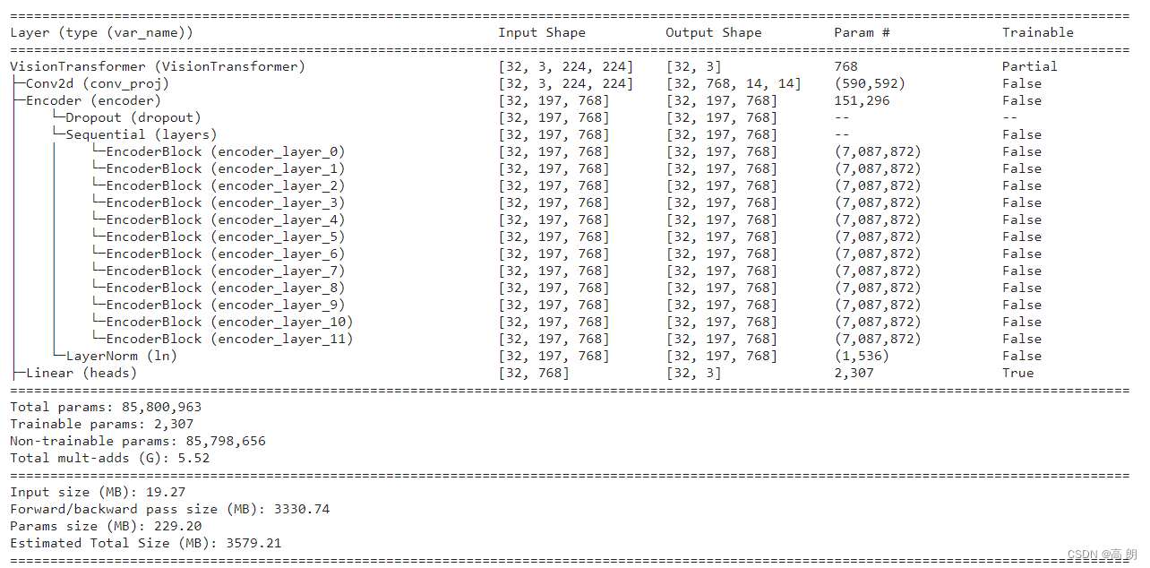 只有输出层是可训练的,而所有其余层都是不可训练的(冻结)。
参数总数为 85,800,963,与上面我们定制的 ViT 模型相同,但是 pretrained_vit 的可训练参数数量比我们自定义的 vit 少得多,只有 2,307 个,而在我们的自定义 vit 中,有 85,800,963 个参数(在我们的自定义 vit 中,因为我们’从头开始重新训练,所有参数都是可训练的)。
- 为预训练ViT模型准备数据
from helper_functions import download_data

# Download pizza, steak, sushi images from GitHub
image_path = download_data(source="https://github.com/mrdbourke/pytorch-deep-learning/raw/main/data/pizza_steak_sushi.zip",
                           destination="pizza_steak_sushi")
image_path
# Setup train and test directory paths
train_dir = image_path / "train"
test_dir = image_path / "test"
train_dir, test_dir
# Get automatic transforms from pretrained ViT weights
pretrained_vit_transforms = pretrained_vit_weights.transforms()
print(pretrained_vit_transforms)
# Setup dataloaders
train_dataloader_pretrained, test_dataloader_pretrained, class_names = data_setup.create_dataloaders(train_dir=train_dir,
                                                                                                     test_dir=test_dir,
                                                                                                     transform=pretrained_vit_transforms,
                                                                                                     batch_size=32) # Could increase if we had more samples, such as here: https://arxiv.org/abs/2205.01580 (there are other improvements there too...)
- 训练特征提取器ViT模型
特征提取器模型准备就绪,数据加载器准备就绪,开始训练:
from going_modular.going_modular import engine

# Create optimizer and loss function
optimizer = torch.optim.Adam(params=pretrained_vit.parameters(),
                             lr=1e-3)
loss_fn = torch.nn.CrossEntropyLoss()

# Train the classifier head of the pretrained ViT feature extractor model
set_seeds()
pretrained_vit_results = engine.train(model=pretrained_vit,
                                      train_dataloader=train_dataloader_pretrained,
                                      test_dataloader=test_dataloader_pretrained,
                                      optimizer=optimizer,
                                      loss_fn=loss_fn,
                                      epochs=10,
                                      device=device)
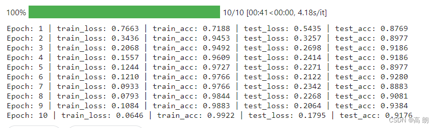
- 绘制特征提取器ViT模型损失曲线
# Plot the loss curves
from helper_functions import plot_loss_curves

plot_loss_curves(pretrained_vit_results)
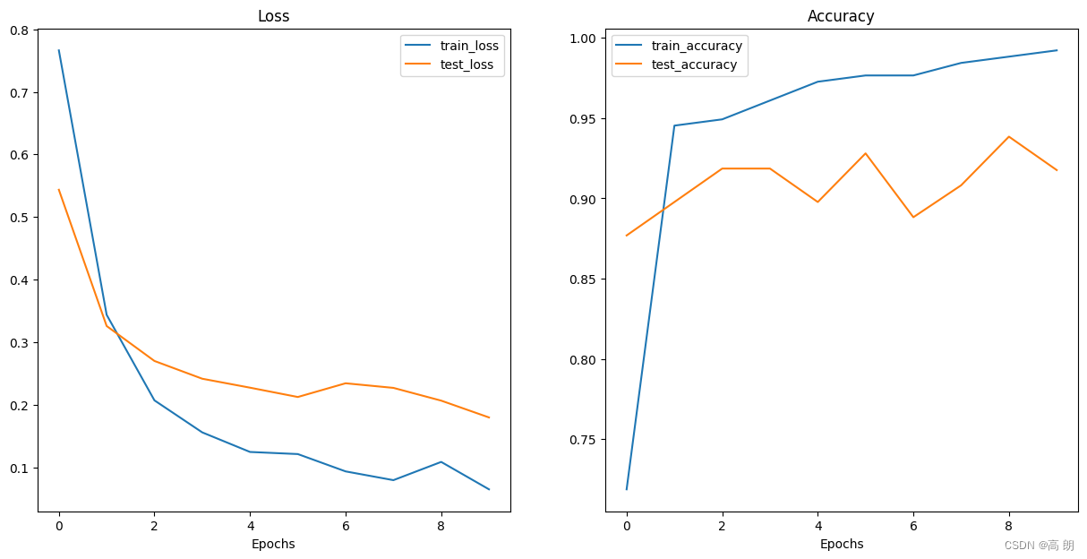
- 保存特征提取器ViT模型并检查文件大小
# Save the model
from going_modular.going_modular import utils

utils.save_model(model=pretrained_vit,
                 target_dir="models",
                 model_name="08_pretrained_vit_feature_extractor_pizza_steak_sushi.pth")
from pathlib import Path

# Get the model size in bytes then convert to megabytes
pretrained_vit_model_size = Path("models/08_pretrained_vit_feature_extractor_pizza_steak_sushi.pth").stat().st_size // (1024*1024) # division converts bytes to megabytes (roughly)
print(f"Pretrained ViT feature extractor model size: {pretrained_vit_model_size} MB")
Pretrained ViT feature extractor model size: 327 MB
11. 对自定义图像进行预测
随机选择一张图片进行预测:
import requests

# Import function to make predictions on images and plot them
from going_modular.going_modular.predictions import pred_and_plot_image

# Setup custom image path
custom_image_path = image_path / "04-pizza-dad.jpeg"

# Download the image if it doesn't already exist
if not custom_image_path.is_file():
    with open(custom_image_path, "wb") as f:
        # When downloading from GitHub, need to use the "raw" file link
        request = requests.get("https://raw.githubusercontent.com/mrdbourke/pytorch-deep-learning/main/images/04-pizza-dad.jpeg")
        print(f"Downloading {custom_image_path}...")
        f.write(request.content)
else:
    print(f"{custom_image_path} already exists, skipping download.")

# Predict on custom image
pred_and_plot_image(model=pretrained_vit,
                    image_path=custom_image_path,
                    class_names=class_names)


 9410
9410

 被折叠的 条评论
为什么被折叠?
被折叠的 条评论
为什么被折叠?
 到【灌水乐园】发言


