【Pytorch】Transfer Learning 迁移学习

最新推荐文章于 2024-07-16 11:42:34 发布

高朗

最新推荐文章于 2024-07-16 11:42:34 发布

阅读量635

点赞数 8

分类专栏： pytorch 文章标签： pytorch 迁移学习人工智能

本文链接：https://blog.csdn.net/qq_43466788/article/details/136315495

版权

pytorch 专栏收录该内容

14 篇文章 4 订阅

订阅专栏

文章目录

1. 获取数据
2. 创建Dataset和DataLoader
3. 获取预训练模型
4. 训练模型
5. 通过绘制损失曲线来评估模型
6. 对测试集中的图像进行预测
补充

迁移学习允许我们采用另一个模型从另一个问题中学到的模式（也称为权重）并将它们用于我们自己的问题。

例如，我们可以采用计算机视觉模型从 ImageNet（数百万张不同对象的图像）等数据集学习到的模式，并使用它们来为我们自己的模型提供支持。也可以从语言模型（通过大量文本来学习语言表示的模型）中获取模式，并将它们用作模型的基础来对不同的文本样本进行分类。

总的一点，找到一个性能良好的现有模型并将其应用于自己的问题。

怎么去找这些已经训练好的模型，即预训练模型：

名称	介绍	Link(s) 链接
PyTorch domain libraries	每个 PyTorch domain libraries（ torchvision 、 torchtext ）都附带某种形式的预训练模型。那里的模型可以在 PyTorch 中运行。	torchvision.models, torchtext.models, torchaudio.models, torchrec.models
HuggingFace Hub	来自世界各地的组织针对许多不同领域（视觉、文本、音频等）的一系列预训练模型。还有很多不同的数据集。	https://huggingface.co/models https://huggingface.co/datasets
timm （PyTorch 图像模型）库	PyTorch 代码中几乎所有最新、最好的计算机视觉模型以及许多其他有用的计算机视觉功能。	https://github.com/rwightman/pytorch-image-models
Paperswithcode	最新最先进的机器学习论文的集合，并附有代码实现。您还可以在此处找到不同任务的模型性能基准。	https://paperswithcode.com/

有了上述高质量的资源，在解决每个深度学习问题时，问“我的问题是否存在预训练模型？”应该是一种常见的做法。

我们将从 torchvision.models 中获取一个预训练模型，并对其进行自定义以解决（并希望改进）我们的 FoodVision Mini 问题。

FoodVision Mini 问题来着【Pytorch】处理自定义数据集，我们自己设计的模型表现很差，采用预训练模型来解决这个问题，主要步骤如下：【数据集来源参考上面链接】

获取数据
创建Dataset和DataLoader
获取并定制预训练模型
训练模型
通过绘制损失曲线来评估模型
对测试集中的图像进行预测

在进行上面操作时，需要进行如下设置：【导入所需的模块】

为了节省文章篇幅，将会利用【Pytorch】模块化中创建的一些 Python 脚本（例如 data_setup.py 和 engine.py ）。
关于torch 和torchvision 的版本需求：torch >= 1.12 和 torchvision >= 0.13

# Continue with regular imports

import matplotlib.pyplot as plt
import torch
import torchvision

from torch import nn
from torchvision import transforms
from torchinfo import summary

from going_modular.going_modular import data_setup, engine

# Setup device agnostic code
device = "cuda" if torch.cuda.is_available() else "cpu"
device

1. 获取数据

参考【Pytorch】处理自定义数据集里面的数据获取。

也可以直接参考下面代码下载数据集：

import os
import zipfile

from pathlib import Path

import requests

# Setup path to data folder
data_path = Path("data/")
image_path = data_path / "pizza_steak_sushi"

# If the image folder doesn't exist, download it and prepare it... 
if image_path.is_dir():
    print(f"{image_path} directory exists.")
else:
    print(f"Did not find {image_path} directory, creating one...")
    image_path.mkdir(parents=True, exist_ok=True)
    
    # Download pizza, steak, sushi data
    with open(data_path / "pizza_steak_sushi.zip", "wb") as f:
        request = requests.get("https://github.com/mrdbourke/pytorch-deep-learning/raw/main/data/pizza_steak_sushi.zip")
        print("Downloading pizza, steak, sushi data...")
        f.write(request.content)

    # Unzip pizza, steak, sushi data
    with zipfile.ZipFile(data_path / "pizza_steak_sushi.zip", "r") as zip_ref:
        print("Unzipping pizza, steak, sushi data...") 
        zip_ref.extractall(image_path)

    # Remove .zip file
    os.remove(data_path / "pizza_steak_sushi.zip")

# Setup Dirs
train_dir = image_path / "train"
test_dir = image_path / "test"

2. 创建Dataset和DataLoader

DataLoader创建参考【Pytorch】模块化中data_setup.py

根据 torchvision的版本选择 1. 手动创建和 2. 自动创建

在 torchvision v0.13+ 之前，使用 torchvision.models 中的预训练模型，因此我们需要首先准备图像的特定转换：

创建 torchvision.models 的转换（手动创建）【torchvision v < 0.13】

使用预训练模型时，重要的是要以与进入模型的原始训练数据相同的方式准备进入模型的自定义数据。
在 torchvision v0.13+ 之前，要为 torchvision.models 中的预训练模型创建转换，文档指出：【可以通过以下组合来实现上述转变】

Transform number	Transform required	Code to perform transform
1	大小为 [batch_size, 3, height, width] 的小批量，其中高度和宽度至少为 224x224。	`torchvision.transforms.Resize()` 将图像大小调整为 [3, 224, 224] 和 `torch.utils.data.DataLoader()` 以创建批量图像。
2	值介于 0 和 1 之间。	`torchvision.transforms.ToTensor()`
3	[0.485, 0.456, 0.406] 的平均值（每个颜色通道的值）。	`torchvision.transforms.Normalize(mean=...)` 调整图像的平均值。
4	标准差为 [0.229, 0.224, 0.225] （每个颜色通道的值）。	`torchvision.transforms.Normalize(std=...)` 调整图像的标准偏差。

完整操作代码：

# Create a transforms pipeline manually (required for torchvision < 0.13)
manual_transforms = transforms.Compose([
    transforms.Resize((224, 224)), # 1. Reshape all images to 224x224 (though some models may require different sizes)
    transforms.ToTensor(), # 2. Turn image values to between 0 & 1 
    transforms.Normalize(mean=[0.485, 0.456, 0.406], # 3. A mean of [0.485, 0.456, 0.406] (across each colour channel)
                         std=[0.229, 0.224, 0.225]) # 4. A standard deviation of [0.229, 0.224, 0.225] (across each colour channel),
])

下面直接调用data_setup.py 脚本中的 create_dataloaders 函数来创建DataLoader:

# Create training and testing DataLoaders as well as get a list of class names
train_dataloader, test_dataloader, class_names = data_setup.create_dataloaders(train_dir=train_dir,
                                                                               test_dir=test_dir,
                                                                               transform=manual_transforms, # resize, convert images to between 0 & 1 and normalize them
                                                                               batch_size=32) # set mini-batch size to 32

train_dataloader, test_dataloader, class_names

为 torchvision.models 创建转换（自动创建）【torchvision v >= 0.13】
在使用预训练模型时，重要的是要以与进入模型的原始训练数据相同的方式准备进入模型的自定义数据。

从 torchvision v0.13+ 开始，添加了自动变换创建功能。

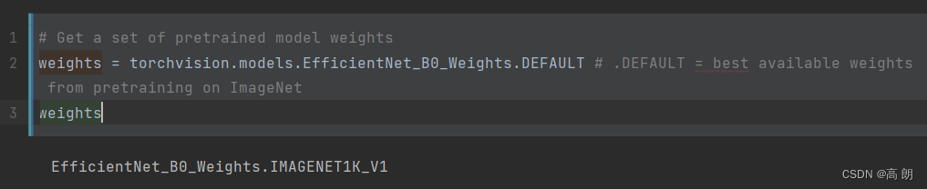
从 torchvision.models 设置模型并选择您想要使用的预训练模型权重：
weights = torchvision.models.EfficientNet_B0_Weights.DEFAULT

EfficientNet_B0_Weights 是我们想要使用的模型架构权重（ torchvision.models 中有许多不同的模型架构选项）。
DEFAULT 表示最佳可用权重（ImageNet 中的最佳性能）。

# Get a set of pretrained model weights
weights = torchvision.models.EfficientNet_B0_Weights.DEFAULT # .DEFAULT = best available weights from pretraining on ImageNet
weights

在这里插入图片描述现在要访问与 weights 相关的转换，我们可以使用 transforms() 方法:

# Get the transforms used to create our pretrained weights
auto_transforms = weights.transforms()
auto_transforms

在这里插入图片描述像前面一样使用 auto_transforms 使用 create_dataloaders() 创建 DataLoaders:

# Create training and testing DataLoaders as well as get a list of class names
train_dataloader, test_dataloader, class_names = data_setup.create_dataloaders(train_dir=train_dir,
                                                                               test_dir=test_dir,
                                                                               transform=auto_transforms, # perform same data transforms on our own data as the pretrained model
                                                                               batch_size=32) # set mini-batch size to 32

train_dataloader, test_dataloader, class_names

3. 获取预训练模型

有大量常见的计算机视觉架构主干：

在这里插入图片描述

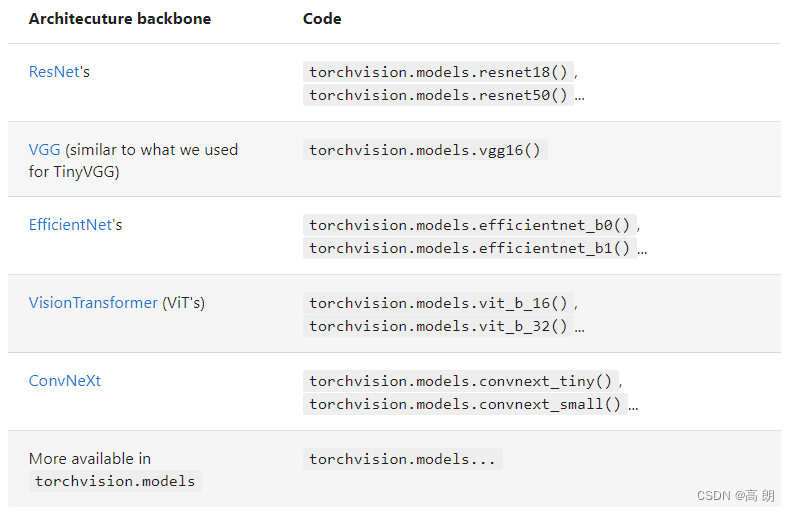
使用哪种预训练模型【取决于你的问题/你正在使用的设备】
一般来说，模型名称中的数字越大（例如 efficientnet_b0() -> efficientnet_b1() -> efficientnet_b7() ）意味着性能更好，但模型更大。
建立预训练模型
使用的预训练模型是 torchvision.models.efficientnet_b0() ：该架构来自论文 EfficientNet: Rethinking Model Scaling for Convolutional Neural Networks。

我们要创建的示例是来自 torchvision.models 的预训练 EfficientNet_B0 模型，其输出层根据我们对披萨、牛排和寿司图像进行分类的用例进行了调整。

我们可以使用与创建转换相同的代码来设置 EfficientNet_B0 预训练的 ImageNet 权重。这意味着该模型已经过数百万张图像的训练，并且具有良好的图像数据基础表示。

该预训练模型的 PyTorch 版本能够在 ImageNet 的 1000 个类别中实现约 77.7% 的准确率

还可以将其发送到目标设备：

# OLD: Setup the model with pretrained weights and send it to the target device (this was prior to torchvision v0.13)
# model = torchvision.models.efficientnet_b0(pretrained=True).to(device) # OLD method (with pretrained=True)

# NEW: Setup the model with pretrained weights and send it to the target device (torchvision v0.13+)
weights = torchvision.models.EfficientNet_B0_Weights.DEFAULT # .DEFAULT = best available weights
model = torchvision.models.efficientnet_b0(weights=weights).to(device)

#model # uncomment to output (it's very long)

在这里插入图片描述这个模型有很多很多很多层。

这是迁移学习的好处之一，它采用现有的模型，该模型是由世界上一些最好的工程师精心设计的，并应用于你自己的问题。

efficientnet_b0 分为三个主要部分：

（1）features - 卷积层和其他各种激活层的集合，用于学习视觉数据的基本表示（此基本表示/层集合通常称为特征或特征提取器，“视觉数据的基本层”，模型学习图像的不同特征）。
（2）avgpool - 取 features 层输出的平均值并将其转换为特征向量。
（3）classifier - 将特征向量转换为与所需输出类数量具有相同维度的向量（因为 efficientnet_b0 是在 ImageNet 上预训练的，并且 ImageNet 有 1000 个类， out_features=1000

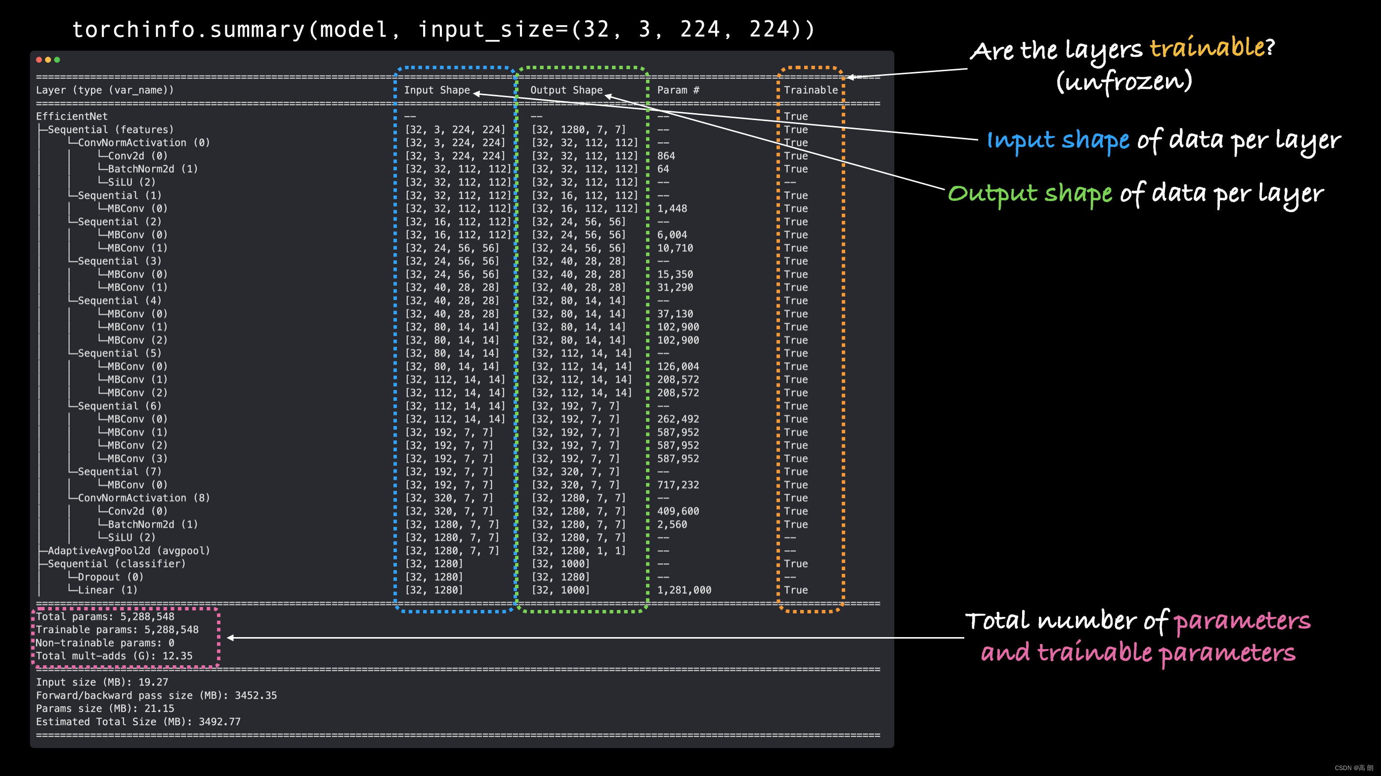
使用 torchinfo.summary() 获取模型摘要

要了解有关模型的更多信息，可以使用 torchinfo 的 summary() 方法。
需要传入：

model - 我们想要获取摘要的模型。
input_size - 我们想要传递给模型的数据的形状，对于 efficientnet_b0 的情况，输入大小为 (batch_size, 3, 224, 224) ，尽管还有其他变体 efficientnet_bX 的输入大小不同。
col_names - 我们希望看到的有关模型的各种信息列。
col_width - 摘要的列应有多宽。
row_settings - 连续显示哪些功能

# Print a summary using torchinfo (uncomment for actual output)
summary(model=model, 
        input_size=(32, 3, 224, 224), # make sure this is "input_size", not "input_shape"
        # col_names=["input_size"], # uncomment for smaller output
        col_names=["input_size", "output_size", "num_params", "trainable"],
        col_width=20,
        row_settings=["var_names"]
)

在这里插入图片描述

将基础模型冻结并更改输出层以适应我们的需求

迁移学习的过程通常是这样的：冻结预训练模型的一些基础层（通常是 features 部分），然后调整输出层（也称为头/分类器层）以满足您的需求。
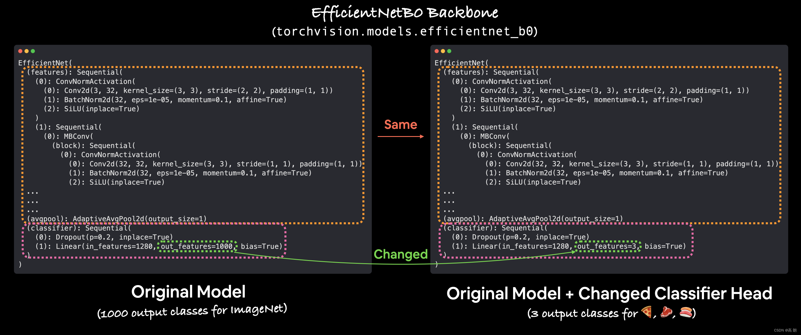在这里插入图片描述可以通过更改输出层来自定义预训练模型的输出以满足您的问题。原始的 torchvision.models.efficientnet_b0() 带有 out_features=1000 ，因为 ImageNet 中有 1000 个类，它是训练的数据集。然而，对于我们的问题，对披萨、牛排和寿司的图像进行分类，我们只需要 out_features=3 。

冻结 efficientnet_b0 模型的 features 部分中的所有层/参数。【冻结图层意味着保持它们在训练期间的原样。例如，如果您的模型具有预训练层，那么冻结它们就是说，“在训练期间不要更改这些层中的任何模式，保持它们的原样。”本质上，我们希望保留我们的模型从 ImageNet 学到的预训练权重/模式作为主干，然后只更改输出层。】

我们可以通过设置属性 requires_grad=False 来冻结 features 部分中的所有图层/参数。

对于带有 requires_grad=False 的参数，PyTorch 不会跟踪梯度更新，反过来，我们的优化器在训练期间也不会更改这些参数。

本质上，具有 requires_grad=False 的参数是“无法训练的”或“冻结”的。

# Freeze all base layers in the "features" section of the model (the feature extractor) by setting requires_grad=False
for param in model.features.parameters():
    param.requires_grad = False

根据需要调整输出层或预训练模型的 classifier 部分：
【现在我们的预训练模型有 out_features=1000 因为 ImageNet 中有 1000 个类。然而，我们没有1000个类，我们只有三个，披萨，牛排和寿司。可以通过创建一系列新的层来更改模型的 classifier 部分。】
当前classifier：

(classifier): Sequential(
    (0): Dropout(p=0.2, inplace=True)
    (1): Linear(in_features=1280, out_features=1000, bias=True)

使用 torch.nn.Dropout(p=0.2, inplace=True)保持 Dropout 层相同。

注意：Dropout 层以 p 的概率随机删除两个神经网络层之间的连接。例如，如果 p=0.2 ，则每次传递都会随机删除神经网络层之间 20% 的连接。这种做法的目的是通过确保保留的连接学习特征来补偿其他连接的删除（希望这些剩余的特征更通用），从而帮助规范化（防止过度拟合）模型。

保留 in_features=1280 作为 Linear 输出层，但将 out_features 值更改为 class_names 的长度（ len([‘pizza’, ‘steak’, ‘sushi’]) = 3 ）.
修改后的代码：

# Set the manual seeds
torch.manual_seed(42)
torch.cuda.manual_seed(42)

# Get the length of class_names (one output unit for each class)
output_shape = len(class_names)

# Recreate the classifier layer and seed it to the target device
model.classifier = torch.nn.Sequential(
    torch.nn.Dropout(p=0.2, inplace=True), 
    torch.nn.Linear(in_features=1280, 
                    out_features=output_shape, # same number of output units as our number of classes
                    bias=True)).to(device)

再次通过summary方法查看模型摘要：

# # Do a summary *after* freezing the features and changing the output classifier layer (uncomment for actual output)
summary(model,
        input_size=(32, 3, 224, 224), # make sure this is "input_size", not "input_shape" (batch_size, color_channels, height, width)
        verbose=0,
        col_names=["input_size", "output_size", "num_params", "trainable"],
        col_width=20,
        row_settings=["var_names"]
)

在这里插入图片描述有以下变化：

可训练列Trainable column - 您将看到许多基础层（ features 部分中的层）的可训练值为 False 。这是因为我们设置了它们的属性 requires_grad=False 。除非我们改变这一点，否则这些层在未来的训练期间不会更新。
classifier 的输出形状 - 模型的 classifier 部分现在的输出形状值为 [32, 3] 而不是 [32, 1000] 。它的可训练值也是 True 。这意味着它的参数将在训练期间更新。本质上，我们使用 features 部分为 classifier 部分提供图像的基本表示，然后我们的 classifier 层将学习如何基本表示与我们的问题相符。
可训练参数较少 - 之前有 5,288,548 个可训练参数。但由于我们冻结了模型的许多层，只留下 classifier 可训练，因此现在只有 3,843 个可训练参数（甚至比我们的 TinyVGG 模型还要少）。尽管还有 4,007,548 个不可训练参数，但这些参数将创建输入图像的基本表示，以馈送到我们的 classifier 层中。

注意：模型的可训练参数越多，计算能力就越强/训练时间就越长。冻结模型的基础层并保留较少的可训练参数意味着我们的模型应该训练得相当快。这是迁移学习的一大好处，它采用针对与您的问题类似的问题训练的模型的已学习参数，并且仅稍微调整输出以适应您的问题。

4. 训练模型

已经有了一个半冻结的预训练模型，并且有一个定制的 classifier。
为了开始训练，我们创建一个损失函数和一个优化器：

# Define loss and optimizer
loss_fn = nn.CrossEntropyLoss()
optimizer = torch.optim.Adam(model.parameters(), lr=0.001)

我们只会在这里训练参数 classifier ，因为模型中的所有其他参数都已被冻结。

# Set the random seeds
torch.manual_seed(42)
torch.cuda.manual_seed(42)

# Start the timer
from timeit import default_timer as timer 
start_time = timer()

# Setup training and save the results
results = engine.train(model=model,
                       train_dataloader=train_dataloader,
                       test_dataloader=test_dataloader,
                       optimizer=optimizer,
                       loss_fn=loss_fn,
                       epochs=5,
                       device=device)

# End the timer and print out how long it took
end_time = timer()
print(f"[INFO] Total training time: {end_time-start_time:.3f} seconds")

在这里插入图片描述
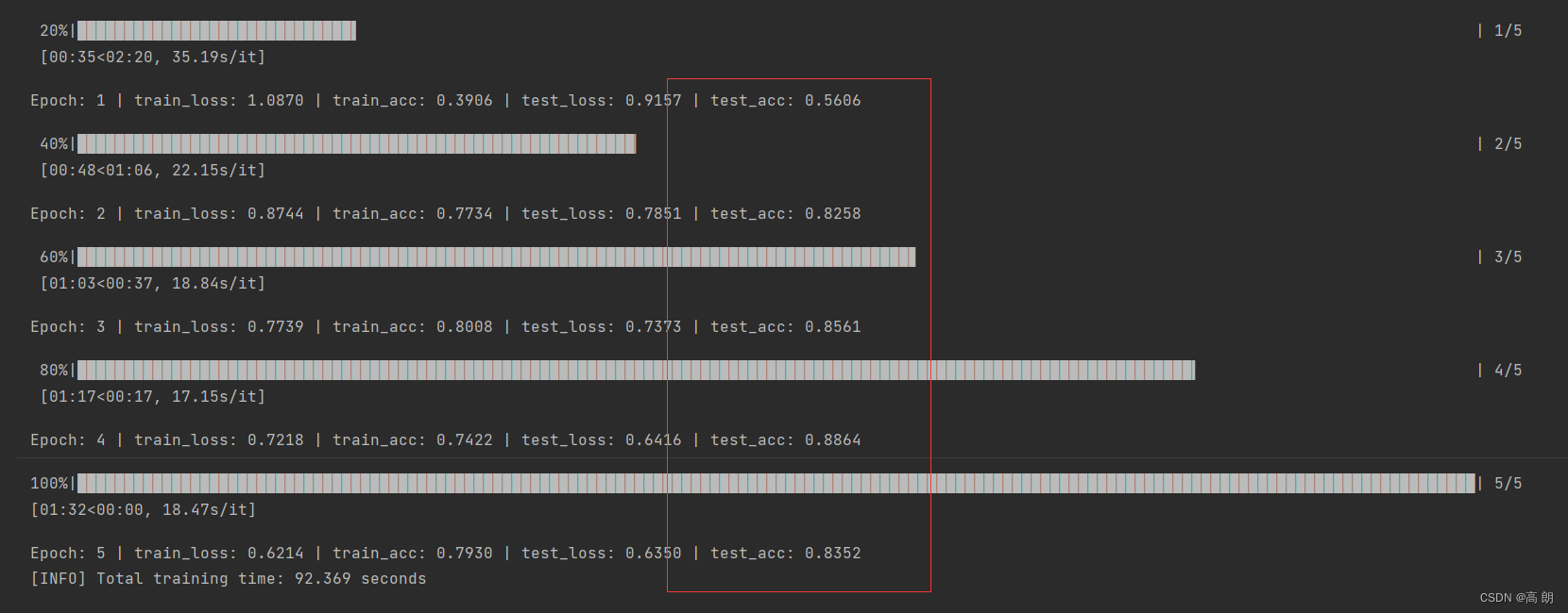
正确率非常高，比自己设计的model要好很多很多。

5. 通过绘制损失曲线来评估模型

绘制损失曲线的脚本helper_functions.py：

"""
A series of helper functions used throughout the course.

If a function gets defined once and could be used over and over, it'll go in here.
"""
import torch
import matplotlib.pyplot as plt
import numpy as np

from torch import nn

import os
import zipfile

from pathlib import Path

import requests

# Walk through an image classification directory and find out how many files (images)
# are in each subdirectory.
import os

def walk_through_dir(dir_path):
    """
    Walks through dir_path returning its contents.
    Args:
    dir_path (str): target directory

    Returns:
    A print out of:
      number of subdiretories in dir_path
      number of images (files) in each subdirectory
      name of each subdirectory
    """
    for dirpath, dirnames, filenames in os.walk(dir_path):
        print(f"There are {len(dirnames)} directories and {len(filenames)} images in '{dirpath}'.")

def plot_decision_boundary(model: torch.nn.Module, X: torch.Tensor, y: torch.Tensor):
    """Plots decision boundaries of model predicting on X in comparison to y.

    Source - https://madewithml.com/courses/foundations/neural-networks/ (with modifications)
    """
    # Put everything to CPU (works better with NumPy + Matplotlib)
    model.to("cpu")
    X, y = X.to("cpu"), y.to("cpu")

    # Setup prediction boundaries and grid
    x_min, x_max = X[:, 0].min() - 0.1, X[:, 0].max() + 0.1
    y_min, y_max = X[:, 1].min() - 0.1, X[:, 1].max() + 0.1
    xx, yy = np.meshgrid(np.linspace(x_min, x_max, 101), np.linspace(y_min, y_max, 101))

    # Make features
    X_to_pred_on = torch.from_numpy(np.column_stack((xx.ravel(), yy.ravel()))).float()

    # Make predictions
    model.eval()
    with torch.inference_mode():
        y_logits = model(X_to_pred_on)

    # Test for multi-class or binary and adjust logits to prediction labels
    if len(torch.unique(y)) > 2:
        y_pred = torch.softmax(y_logits, dim=1).argmax(dim=1)  # mutli-class
    else:
        y_pred = torch.round(torch.sigmoid(y_logits))  # binary

    # Reshape preds and plot
    y_pred = y_pred.reshape(xx.shape).detach().numpy()
    plt.contourf(xx, yy, y_pred, cmap=plt.cm.RdYlBu, alpha=0.7)
    plt.scatter(X[:, 0], X[:, 1], c=y, s=40, cmap=plt.cm.RdYlBu)
    plt.xlim(xx.min(), xx.max())
    plt.ylim(yy.min(), yy.max())


# Plot linear data or training and test and predictions (optional)
def plot_predictions(
    train_data, train_labels, test_data, test_labels, predictions=None
):
    """
  Plots linear training data and test data and compares predictions.
  """
    plt.figure(figsize=(10, 7))

    # Plot training data in blue
    plt.scatter(train_data, train_labels, c="b", s=4, label="Training data")

    # Plot test data in green
    plt.scatter(test_data, test_labels, c="g", s=4, label="Testing data")

    if predictions is not None:
        # Plot the predictions in red (predictions were made on the test data)
        plt.scatter(test_data, predictions, c="r", s=4, label="Predictions")

    # Show the legend
    plt.legend(prop={"size": 14})


# Calculate accuracy (a classification metric)
def accuracy_fn(y_true, y_pred):
    """Calculates accuracy between truth labels and predictions.

    Args:
        y_true (torch.Tensor): Truth labels for predictions.
        y_pred (torch.Tensor): Predictions to be compared to predictions.

    Returns:
        [torch.float]: Accuracy value between y_true and y_pred, e.g. 78.45
    """
    correct = torch.eq(y_true, y_pred).sum().item()
    acc = (correct / len(y_pred)) * 100
    return acc


def print_train_time(start, end, device=None):
    """Prints difference between start and end time.

    Args:
        start (float): Start time of computation (preferred in timeit format). 
        end (float): End time of computation.
        device ([type], optional): Device that compute is running on. Defaults to None.

    Returns:
        float: time between start and end in seconds (higher is longer).
    """
    total_time = end - start
    print(f"\nTrain time on {device}: {total_time:.3f} seconds")
    return total_time


# Plot loss curves of a model
def plot_loss_curves(results):
    """Plots training curves of a results dictionary.

    Args:
        results (dict): dictionary containing list of values, e.g.
            {"train_loss": [...],
             "train_acc": [...],
             "test_loss": [...],
             "test_acc": [...]}
    """
    loss = results["train_loss"]
    test_loss = results["test_loss"]

    accuracy = results["train_acc"]
    test_accuracy = results["test_acc"]

    epochs = range(len(results["train_loss"]))

    plt.figure(figsize=(15, 7))

    # Plot loss
    plt.subplot(1, 2, 1)
    plt.plot(epochs, loss, label="train_loss")
    plt.plot(epochs, test_loss, label="test_loss")
    plt.title("Loss")
    plt.xlabel("Epochs")
    plt.legend()

    # Plot accuracy
    plt.subplot(1, 2, 2)
    plt.plot(epochs, accuracy, label="train_accuracy")
    plt.plot(epochs, test_accuracy, label="test_accuracy")
    plt.title("Accuracy")
    plt.xlabel("Epochs")
    plt.legend()


# Pred and plot image function from notebook 04
# See creation: https://www.learnpytorch.io/04_pytorch_custom_datasets/#113-putting-custom-image-prediction-together-building-a-function
from typing import List
import torchvision


def pred_and_plot_image(
    model: torch.nn.Module,
    image_path: str,
    class_names: List[str] = None,
    transform=None,
    device: torch.device = "cuda" if torch.cuda.is_available() else "cpu",
):
    """Makes a prediction on a target image with a trained model and plots the image.

    Args:
        model (torch.nn.Module): trained PyTorch image classification model.
        image_path (str): filepath to target image.
        class_names (List[str], optional): different class names for target image. Defaults to None.
        transform (_type_, optional): transform of target image. Defaults to None.
        device (torch.device, optional): target device to compute on. Defaults to "cuda" if torch.cuda.is_available() else "cpu".
    
    Returns:
        Matplotlib plot of target image and model prediction as title.

    Example usage:
        pred_and_plot_image(model=model,
                            image="some_image.jpeg",
                            class_names=["class_1", "class_2", "class_3"],
                            transform=torchvision.transforms.ToTensor(),
                            device=device)
    """

    # 1. Load in image and convert the tensor values to float32
    target_image = torchvision.io.read_image(str(image_path)).type(torch.float32)

    # 2. Divide the image pixel values by 255 to get them between [0, 1]
    target_image = target_image / 255.0

    # 3. Transform if necessary
    if transform:
        target_image = transform(target_image)

    # 4. Make sure the model is on the target device
    model.to(device)

    # 5. Turn on model evaluation mode and inference mode
    model.eval()
    with torch.inference_mode():
        # Add an extra dimension to the image
        target_image = target_image.unsqueeze(dim=0)

        # Make a prediction on image with an extra dimension and send it to the target device
        target_image_pred = model(target_image.to(device))

    # 6. Convert logits -> prediction probabilities (using torch.softmax() for multi-class classification)
    target_image_pred_probs = torch.softmax(target_image_pred, dim=1)

    # 7. Convert prediction probabilities -> prediction labels
    target_image_pred_label = torch.argmax(target_image_pred_probs, dim=1)

    # 8. Plot the image alongside the prediction and prediction probability
    plt.imshow(
        target_image.squeeze().permute(1, 2, 0)
    )  # make sure it's the right size for matplotlib
    if class_names:
        title = f"Pred: {class_names[target_image_pred_label.cpu()]} | Prob: {target_image_pred_probs.max().cpu():.3f}"
    else:
        title = f"Pred: {target_image_pred_label} | Prob: {target_image_pred_probs.max().cpu():.3f}"
    plt.title(title)
    plt.axis(False)

def set_seeds(seed: int=42):
    """Sets random sets for torch operations.

    Args:
        seed (int, optional): Random seed to set. Defaults to 42.
    """
    # Set the seed for general torch operations
    torch.manual_seed(seed)
    # Set the seed for CUDA torch operations (ones that happen on the GPU)
    torch.cuda.manual_seed(seed)

def download_data(source: str, 
                  destination: str,
                  remove_source: bool = True) -> Path:
    """Downloads a zipped dataset from source and unzips to destination.

    Args:
        source (str): A link to a zipped file containing data.
        destination (str): A target directory to unzip data to.
        remove_source (bool): Whether to remove the source after downloading and extracting.
    
    Returns:
        pathlib.Path to downloaded data.
    
    Example usage:
        download_data(source="https://github.com/mrdbourke/pytorch-deep-learning/raw/main/data/pizza_steak_sushi.zip",
                      destination="pizza_steak_sushi")
    """
    # Setup path to data folder
    data_path = Path("data/")
    image_path = data_path / destination

    # If the image folder doesn't exist, download it and prepare it... 
    if image_path.is_dir():
        print(f"[INFO] {image_path} directory exists, skipping download.")
    else:
        print(f"[INFO] Did not find {image_path} directory, creating one...")
        image_path.mkdir(parents=True, exist_ok=True)
        
        # Download pizza, steak, sushi data
        target_file = Path(source).name
        with open(data_path / target_file, "wb") as f:
            request = requests.get(source)
            print(f"[INFO] Downloading {target_file} from {source}...")
            f.write(request.content)

        # Unzip pizza, steak, sushi data
        with zipfile.ZipFile(data_path / target_file, "r") as zip_ref:
            print(f"[INFO] Unzipping {target_file} data...") 
            zip_ref.extractall(image_path)

        # Remove .zip file
        if remove_source:
            os.remove(data_path / target_file)
    
    return image_path

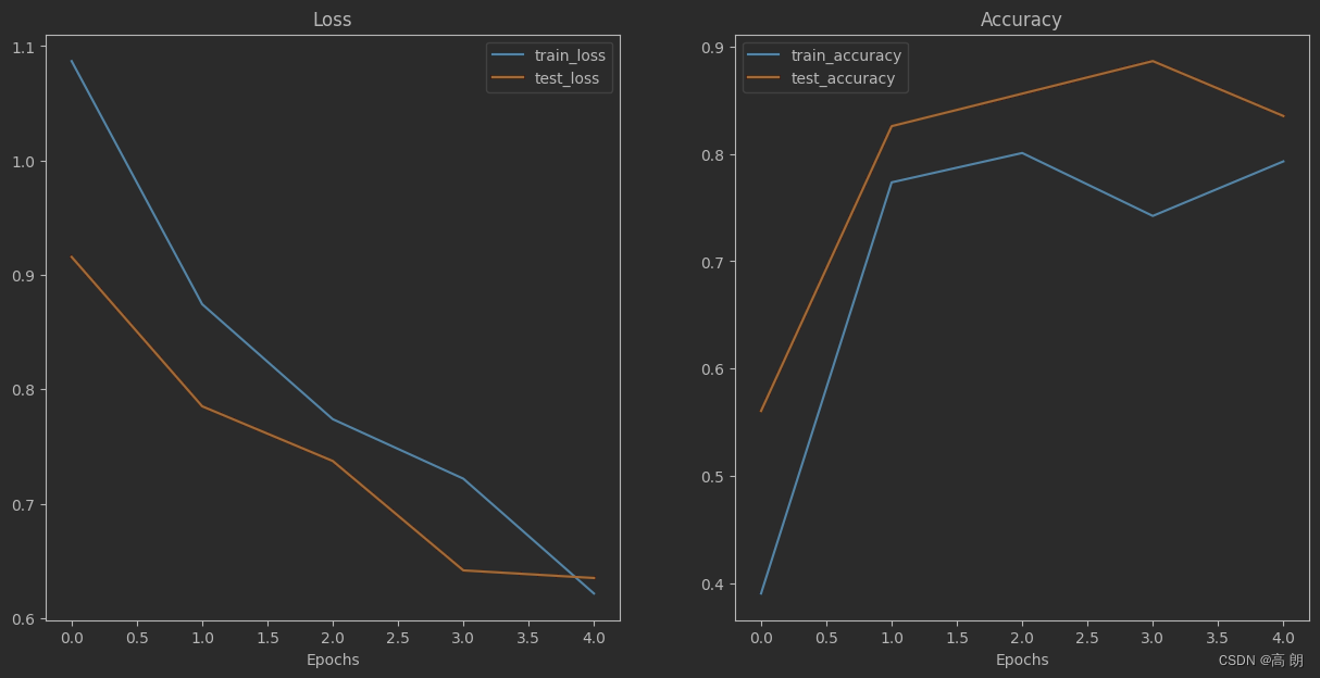
导入notebook并绘制：

from helper_functions import plot_loss_curves

# Plot the loss curves of our model
plot_loss_curves(results)

在这里插入图片描述

6. 对测试集中的图像进行预测

必须记住的一件事是，为了让我们的模型对图像进行预测，该图像必须与我们的模型所训练的图像具有相同的格式。
（1）相同的形状 - 如果我们的图像与模型训练时的形状不同，我们会得到形状错误。
（2）相同的数据类型 - 如果我们的图像是不同的数据类型（例如 torch.int8 与 torch.float32 ），我们将收到数据类型错误.
（3）相同的设备 - 如果我们的图像与我们的模型位于不同的设备上，我们将收到设备错误。
（4）相同的转换 - 如果我们的模型是在以某种方式转换的图像上进行训练的（例如，用特定的平均值和标准差进行标准化），并且我们尝试对以不同方式转换的图像进行预测，那么这些预测可能会失败。

将上面整合成一个函数pred_and_plot_image() :

需要的参数：经过训练的模型、类名列表、目标图像的文件路径、图像大小、转换和目标设备。
使用 PIL.Image.open() 打开图像。
为图像创建一个转换（这将默认为我们上面创建的 manual_transforms 或者它可以使用从 weights.transforms() 生成的转换）。
确保该模型位于目标设备上。
使用 model.eval() 打开模型评估模式（这会关闭 nn.Dropout() 等层，因此它们不用于推理）和推理模式上下文管理器。
使用步骤 3 中进行的变换来变换目标图像，并使用 torch.unsqueeze(dim=0) 添加额外的批量维度，以便我们的输入图像具有形状 [batch_size, color_channels, height, width] 。
通过将图像传递给模型来对图像进行预测，确保它位于目标设备上。
使用 torch.softmax() 将模型的输出 logits 转换为预测概率。
使用 torch.argmax() 将模型的预测概率转换为预测标签。
使用 matplotlib 绘制图像，并将标题设置为步骤 9 中的预测标签和步骤 8 中的预测概率。

from typing import List, Tuple

from PIL import Image

# 1. Take in a trained model, class names, image path, image size, a transform and target device
def pred_and_plot_image(model: torch.nn.Module,
                        image_path: str, 
                        class_names: List[str],
                        image_size: Tuple[int, int] = (224, 224),
                        transform: torchvision.transforms = None,
                        device: torch.device=device):
    
    
    # 2. Open image
    img = Image.open(image_path)

    # 3. Create transformation for image (if one doesn't exist)
    if transform is not None:
        image_transform = transform
    else:
        image_transform = transforms.Compose([
            transforms.Resize(image_size),
            transforms.ToTensor(),
            transforms.Normalize(mean=[0.485, 0.456, 0.406],
                                 std=[0.229, 0.224, 0.225]),
        ])

    ### Predict on image ### 

    # 4. Make sure the model is on the target device
    model.to(device)

    # 5. Turn on model evaluation mode and inference mode
    model.eval()
    with torch.inference_mode():
      # 6. Transform and add an extra dimension to image (model requires samples in [batch_size, color_channels, height, width])
      transformed_image = image_transform(img).unsqueeze(dim=0)

      # 7. Make a prediction on image with an extra dimension and send it to the target device
      target_image_pred = model(transformed_image.to(device))

    # 8. Convert logits -> prediction probabilities (using torch.softmax() for multi-class classification)
    target_image_pred_probs = torch.softmax(target_image_pred, dim=1)

    # 9. Convert prediction probabilities -> prediction labels
    target_image_pred_label = torch.argmax(target_image_pred_probs, dim=1)

    # 10. Plot image with predicted label and probability 
    plt.figure()
    plt.imshow(img)
    plt.title(f"Pred: {class_names[target_image_pred_label]} | Prob: {target_image_pred_probs.max():.3f}")
    plt.axis(False);

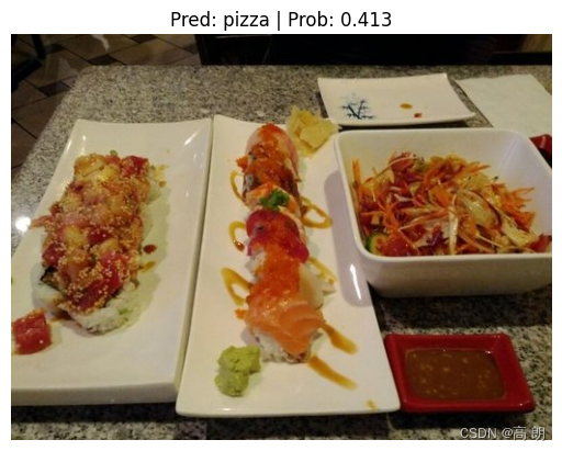
测试：
使用list(Path(test_dir).glob("*/*.jpg")) 获取所有测试图像路径的列表， glob() 方法中的星星表示“匹配此模式的任何文件”，换句话说，任何以 < .jpg>（我们所有的图像）。
可以使用 Python 的 random.sample(populuation, k) 随机采样其中的多个，其中 population 是要采样的序列， k 是要检索的样本数量。

# Get a random list of image paths from test set
import random
num_images_to_plot = 3
test_image_path_list = list(Path(test_dir).glob("*/*.jpg")) # get list all image paths from test data 
test_image_path_sample = random.sample(population=test_image_path_list, # go through all of the test image paths
                                       k=num_images_to_plot) # randomly select 'k' image paths to pred and plot

# Make predictions on and plot the images
for image_path in test_image_path_sample:
    pred_and_plot_image(model=model, 
                        image_path=image_path,
                        class_names=class_names,
                        # transform=weights.transforms(), # optionally pass in a specified transform from our pretrained model weights
                        image_size=(224, 224))

在这里插入图片描述

在这里插入图片描述
对自定义的图片进行测试，例如随便找的下面图片：

# Setup custom image path
custom_image_path = data_path / "predicate/04-pizza-dad.jpeg"

# Predict on custom image
pred_and_plot_image(model=model,
                    image_path=custom_image_path,
                    class_names=class_names)

在这里插入图片描述

补充

上面对测试集是随机选取几张进行测试，补充对全部测试集进行预测：

from tqdm.auto import tqdm

# Make predictions on the entire test dataset
test_preds = []
model.eval()
with torch.inference_mode():
  # Loop through the batches in the test dataloader
  for X, y in tqdm(test_dataloader):
    X, y = X.to(device), y.to(device)
    # Pass the data through the model
    test_logits = model(X)

    # Convert the pred logits to pred probs
    pred_probs = torch.softmax(test_logits, dim=1)

    # Convert the pred probs into pred labels
    pred_labels = torch.argmax(pred_probs, dim=1)

    # Add the pred labels to test preds list
    test_preds.append(pred_labels)

# Concatenate the test preds and put them on the CPU
test_preds = torch.cat(test_preds).cpu()
test_preds

在这里插入图片描述
2. 使用测试预测和真值标签制作混淆矩阵
需要用到的库：torchmetrics, mlxtend
下载命令：!pip install -q torchmetrics -U mlxtend
拿到真值标签：

# Get the truth labels for test dataset
test_truth = torch.cat([y for X, y in test_dataloader])
test_truth

绘制混淆矩阵：

from torchmetrics import ConfusionMatrix
from mlxtend.plotting import plot_confusion_matrix

# Setup confusion matrix instance
confmat = ConfusionMatrix(task='multiclass', num_classes=len(class_names))
confmat_tensor = confmat(preds=test_preds,
                         target=test_truth)

# Plot the confusion matrix
fig, ax = plot_confusion_matrix(
    conf_mat=confmat_tensor.numpy(), # matplotlib likes working with NumPy
    class_names=class_names,
    figsize=(10, 7)
)

在这里插入图片描述
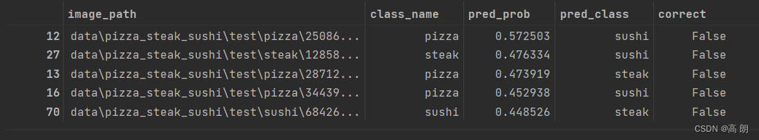
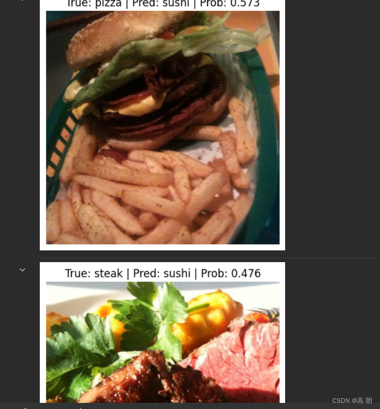
3. 获取测试数据集上“最错误”的预测，并绘制 5 个“最错误”的图像。

对所有测试数据集进行预测，存储标签和预测概率。
按错误预测然后降序预测概率对预测进行排序，这将为您提供具有最高预测概率的错误预测，换句话说，“最错误”。
绘制前 5 个“最错误”的图像，并考虑模型为什么会犯这些错误？

具体操作：

创建一个包含样本、标签、预测、预测概率的 DataFrame
按正确顺序对 DataFrame 进行排序（标签 == 预测）
按预测概率对 DataFrame 进行排序（降序）
绘制前 5 个“最错误”的图

# Get all test data paths
from pathlib import Path
test_data_paths = list(Path(test_dir).glob("*/*.jpg"))
test_labels = [path.parent.stem for path in test_data_paths]

# Create a function to return a list of dictionaries with sample, label, prediction, pred prob
def pred_and_store(test_paths, model, transform, class_names, device):
  test_pred_list = []
  for path in tqdm(test_paths):
    # Create empty dict to store info for each sample
    pred_dict = {}

    # Get sample path
    pred_dict["image_path"] = path

    # Get class name
    class_name = path.parent.stem
    pred_dict["class_name"] = class_name

    # Get prediction and prediction probability
    from PIL import Image
    img = Image.open(path) # open image
    transformed_image = transform(img).unsqueeze(0) # transform image and add batch dimension
    model.eval()
    with torch.inference_mode():
      pred_logit = model(transformed_image.to(device))
      pred_prob = torch.softmax(pred_logit, dim=1)
      pred_label = torch.argmax(pred_prob, dim=1)
      pred_class = class_names[pred_label.cpu()]

      # Make sure things in the dictionary are back on the CPU
      pred_dict["pred_prob"] = pred_prob.unsqueeze(0).max().cpu().item()
      pred_dict["pred_class"] = pred_class

    # Does the pred match the true label?
    pred_dict["correct"] = class_name == pred_class

    # print(pred_dict)
    # Add the dictionary to the list of preds
    test_pred_list.append(pred_dict)

  return test_pred_list

test_pred_dicts = pred_and_store(test_paths=test_data_paths,
                                 model=model,
                                 transform=auto_transforms,
                                 class_names=class_names,
                                 device=device)

test_pred_dicts[:5]

# Turn the test_pred_dicts into a DataFrame
import pandas as pd
test_pred_df = pd.DataFrame(test_pred_dicts)
# Sort DataFrame by correct then by pred_prob
top_5_most_wrong = test_pred_df.sort_values(by=["correct", "pred_prob"], ascending=[True, False]).head()
top_5_most_wrong

在这里插入图片描述

import torchvision
import matplotlib.pyplot as plt
# Plot the top 5 most wrong images
for row in top_5_most_wrong.iterrows():
  row = row[1]
  image_path = row[0]
  true_label = row[1]
  pred_prob = row[2]
  pred_class = row[3]
  # Plot the image and various details
  img = torchvision.io.read_image(str(image_path)) # get image as tensor
  plt.figure()
  plt.imshow(img.permute(1, 2, 0)) # matplotlib likes images in [height, width, color_channels]
  plt.title(f"True: {true_label} | Pred: {pred_class} | Prob: {pred_prob:.3f}")
  plt.axis(False);