数字图像处理作业：一维无损预测压缩 一维游程编码

游程编码算法
基于预测编码的图像压缩方法的研究

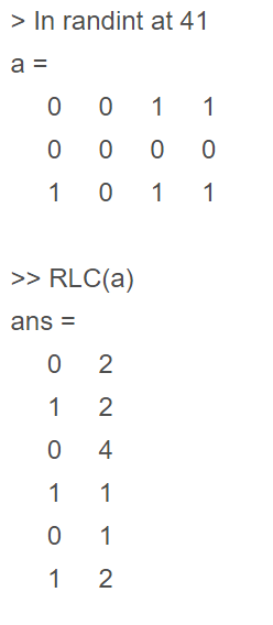
游程编码代码

function S=RLC(I)
%======================================================================================================
% 游程长度编码是栅格数据压缩的重要编码方法，它的基本思路是：对于一幅栅格图像，常常有行(或列)方向上相邻的若干点
% 具有相同的属性代码，因而可采取某种方法压缩那些重复的记录内容。其编码方案是，只在各行(或列)数据的代码发生变化
% 时依次记录该代码以及相同代码重复的个数，从而实现数据的压缩。
%------------------------------------------------------------------------------------------------------
% 例如：5555557777733322221111111 
% 行程编码为：（5，6）（7，5）（3，3）（2，4）（l，7）。
%===================================================================================================
[m,n]=size(I);
if m~=1&&n~=1
    I=I';
    I=reshape(I,1,m*n);
end
j=1;
count=1;
% 对第一个到第m*n个进行一般化处理
for i=1:m*n-1
    if I(i+1)==I(i)
        count=count+1;
    else
       S(j,1)=I(i);
       S(j,2)=count;
       j=j+1;
       count=1;
    end
end
% 最后一个元素处理有两种情况。其一，和前一个元素相等，其二，和前一个元素不等。
% 无论属于哪一种情况都没有在S中记录。
if I(m*n)==I(m*n-1)
    S(j,1)=I(i);
    S(j,2)=count;
else
    S(j,1)=I(m*n);
    S(j,2)=1;
end
% I为字符串
% if m==1||n==1
%     S(:,1)=S(:,1)-'0';
%     S=double(S);
% end
end

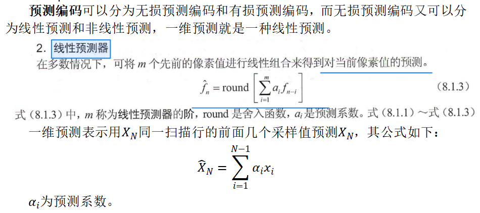
一维预测

下面对大小为512*512像素、灰度级为256的标准lena图像进行无损的一阶预测编码，其matlab程序如下：

I=imread(‘LENA.bmp’);     
x=double(I);
y=LPCencode(x);   
xx=LPCdecode(y);
%显示预测误差值
figure(1);
subplot(121);
imshow(I);
subplot(122);
Imshow(mat2gray(y));
%计算均方差误差，因为是无损编码，那么erms应该为０
e=double(x)-double(xx);
[m, n]=size(e);
erms=sqrt(sum(e(:).^2)/(m*n))    
％显示原图直方图
figure(2);
Subplot(121);
[h, f]=hist(x(:));    
bar(f, h, ‘k’);
%显示预测误差的直方图
subplot(122);
[h, f]=hist(y(:));    
bar(f, h,‘k’);

%编码器
%LPCencode函数用一维无损预测编码压缩图像x,a为预测系数，如果a默认，则默认a=１，就是前值预测。
 function y=LPCencode(x, a)
 error(nargchk(1, 2, nargin));
 if nargin<2
    a=1;
 end
x=double(x);   
[m, n]=size(x);
p=zeros(m, n);  %存放预测值
xs=x;   
zc=zeros(m, 1);
for i=1:length(a)
　　　xs=[zc  xs(:, 1:end-1)];    
　　　p=p+a(i)*xs;
end
y=x-round(p);

%解码器
%LPCdecode函数的解码程序，与编码程序用的是同一个预测器
function x=LPCdecode(y, a)
error(nargchk(1, 2, nargin));
if nargin<2
　　a=1;
 end
 a=a(end: -1: 1);     
[m, n]=size(y);     
order=length(a);
a=repmat(a, m, 1);      
x=zeros(m, n+order);
for i=1:n
 ii=i+order;
x(:, ii)=y(:, i)+round(sum(a(:, order: -1: 1).*x(:, (ii-1): -1:(ii-order)), 2));
end
x=x(:, order+1: end);

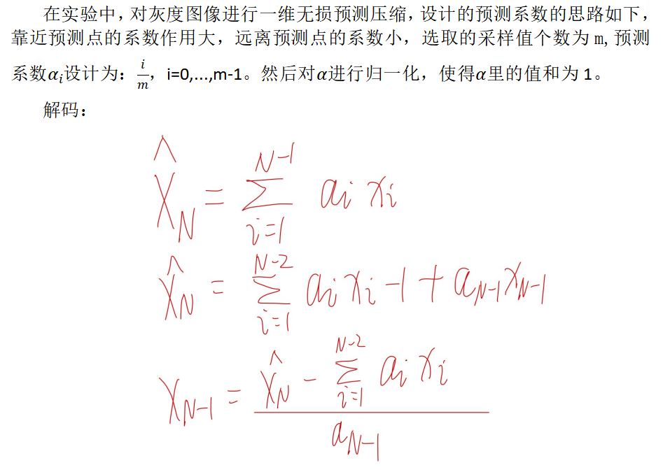
一维预测编码+游程编码 python代码

预测系数设计思路 、解码思路

代码

import cv2 as cv
import numpy as np
from matplotlib import pyplot as plt
# 编码器
# LPCencode函数用一维无损预测编码压缩图像x,a为预测系数，如果a默认，则默认a=１，就是前值预测。
def  LPCencode(x,m,a):
    n=x.shape[0]
    p=np.zeros(n) #存放预测值
    p[0:m]=x[0:m]
    #对后m个点预测
    for i in range(m,n):
     X=x[i-m:i]
     p[i]=np.dot(X,a)

    return np.rint(p) #四舍五入

def  LPCdecode(y,m,a):
    n=y.shape[0]
    x=np.zeros(n) #存放灰度值
    x[0:m]=y[0:m]
    #对后m个点恢复
    for i in range(m,n-1):
     X=x[i-m:i-1]
     p=np.dot(X,a[:m-1])
     x[i]=(y[i+1]-p)/a[m-1]
    x[n-1]=x[n-2]

    return np.rint(x) #四舍五入

def get_mse(records_real, records_predict):
    """
    均方误差 估计值与真值 偏差
    """
    if len(records_real) == len(records_predict):
        return sum([(x - y) ** 2 for x, y in zip(records_real, records_predict)]) / len(records_real)
    else:
        return None

image = cv.imread('2.jpg')
grayimg = cv.cvtColor(image, cv.COLOR_BGR2GRAY)
cv.imwrite('grayImg2.png', grayimg) #保存灰度图
rows, cols = grayimg.shape
image1 = grayimg.flatten() # 把灰度化后的二维图像降维为一维列表
# print(len(image1))

#设计a a的所有值加起来=1
m = 20
a = []
s = (m - 1) / 2
for i in range(m):
    y = i / m / s
    a.append(y)
print('a设计完成,和为',sum(a))

print('预测编码')
img_code=LPCencode(image1,m,a)
pre_image = np.reshape(img_code,(rows,cols)) #预测图像
cv.imwrite('pre_image2.png', pre_image)     #保存

print('预测解码')
img_decode=LPCdecode(img_code,m,a)
de_image = np.reshape(img_decode,(rows,cols)) #预测图像
cv.imwrite('de_image2.png', de_image)     #保存

#计算均方差误差，因为是无损编码，那么erms应该为０
e=image1-img_decode
# print(e)
erms=get_mse(image1,img_decode)
print('均方差误差:',erms)


# 行程压缩编码
data = []
e3 = []
count = 1

for i in range(len(e)-1):
    if (count == 1):
        e3.append(e[i])
    if e[i] == e[i+1]:
        count = count + 1
        if i == len(e) - 2:
            e3.append(e[i])
            data.append(count)
    else:
        data.append(count)
        count = 1

if(e[len(e)-1] != e[-1]):
    e3.append(e[len(e)-1])
    data.append(1)

#计算图像存储空间
size1=rows*cols*8
size2=len(e3)*8
print('压缩前图像存储空间为：',size1,'bit')
print('压缩后图像存储空间为：',size2,'bit')
# 压缩率
ys_rate = (size1-size2)/size1*100
print('压缩率为' + str(ys_rate) + '%')

# 行程编码解码
# rec_e = []
# for i in range(len(data)):
#     for j in range(data[i]):
#         rec_e.append(e3[i])