


import pandas as pd
import os
import numpy as np
HOUSING_PATH = os.path.join("data") # 数据集所在的文件夹
def load_housing_data(housing_path=HOUSING_PATH):
'''
加载数据
Args:
housing_path: 数据集所在的文件夹
Returns:
读取数据
'''
csv_path = os.path.join(housing_path, 'housing.csv') # 数据集路径
return pd.read_csv(csv_path) # 读取数据
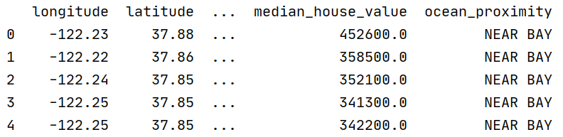
# 查看前五行数据
housing = load_housing_data()
print(housing.head())
# 查看数据集的属性描述信息:总行数,每个属性的类型,非空值数量
print(housing.info())

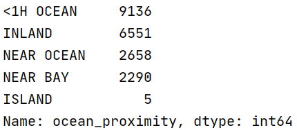
# 查看ocean_proximity属性中有多少分类,每种分类的个数
print(housing['ocean_proximity'].value_counts())
# 显示数据集的数值信息
print(housing.describe())  # 百分比值的意思是:百分之几的数据低于该值

import matplotlib.pyplot as plt

# 绘制每个属性的直方图
housing.hist(bins=50, figsize=(20, 15))  # bins指每个直方图的柱子个数
plt.show()

# 用分层抽样方法创建测试集
# 在数据集中新增一个属性,按照收入多少划分为五个类别,np.inf代表无穷大的浮点正数
housing['income_cat'] = pd.cut(housing['median_income'],
                               bins=[0., 1.5, 3.0, 4.5, 6., np.inf],
                               labels=[1, 2, 3, 4, 5])
# 根据收入类别进行分层抽样
from sklearn.model_selection import StratifiedShuffleSplit

split = StratifiedShuffleSplit(n_splits=1, test_size=0.2, random_state=42)
'''
参数 n_splits是将训练数据分成train/test对的组数,可根据需要进行设置,默认为10
参数test_size和train_size是用来设置train/test对中train和test所占的比例。
random_state控制是将样本随机打乱(42让每一次运行都是一样的随机结果)
'''
for train_index, test_index in split.split(housing, housing["income_cat"]):
    print(train_index, test_index)  # 训练集和测试集的索引号
    strat_train_set = housing.loc[train_index]  # 训练集
    strat_test_set = housing.loc[test_index]  # 测试集

# 查看各收入类别的所占比例
print(strat_train_set['income_cat'].value_counts() / len(strat_train_set))
print(strat_test_set['income_cat'].value_counts() / len(strat_test_set))

# 最后删除辅助属性income_cat
for set_ in (strat_train_set, strat_test_set):
    # 它不改变原有的dataframe中的数据,而是返回另一个dataframe来存放删除后的数据。
    #drop方法有一个可选参数inplace,表明可对原数组作出修改并返回一个新数组。
    #不管参数默认为False还是设置为True,原数组的内存值是不会改变的,区别在于原数组的内容是否直接被修改。
    set_.drop('income_cat', axis=1, inplace=True)

housing = strat_train_set.copy()  # 新创建一个训练集的副本
# 可视化训练集
import matplotlib.image as mpimg

california_img = mpimg.imread(os.path.join('images', 'california.png'))  # 读取加利福尼亚地区图片
# x:经度,y:纬度,alpha:点的不透明度,当点的透明度很高时,单个点的颜色很浅。这样点越密集,对应区域颜色越深。
# s:半径大小(这里代表每个区域人口数量),c=颜色代表价格(红色昂贵,蓝色便宜),cmap:预定义的颜色表
ax = housing.plot(kind="scatter", x="longitude", y="latitude", figsize=(10, 7),
                  s=housing['population'] / 100, label="Population",
                  c="median_house_value", cmap=plt.get_cmap("jet"),
                  colorbar=False, alpha=0.4)
plt.imshow(california_img, extent=[-124.55, -113.80, 32.45, 42.05], alpha=0.5,
           cmap=plt.get_cmap("jet"))  # 按经度纬度截取加利福尼亚的图片
plt.ylabel("Latitude", fontsize=14)
plt.xlabel("Longitude", fontsize=14)
#画旁边的颜色条
prices = housing["median_house_value"]
tick_values = np.linspace(prices.min(), prices.max(), 11)
cbar = plt.colorbar(ticks=tick_values / prices.max())
cbar.ax.set_yticklabels(["$%dk" % (round(v / 1000)) for v in tick_values], fontsize=14)
cbar.set_label('Median House Value', fontsize=16)
plt.legend(fontsize=16)
plt.show()

corr_matrix = housing.corr()  # 获取每对属性之间的标准相关系数
# 查看每个属性与房价中位数的相关性
# 越接近1越代表有较强的正相关性,越接近0代表没有相关性,越接近-1越代表有较强的负相关性。
print(corr_matrix['median_house_value'].sort_values(ascending=False))  # 结果按降序排列
# 绘制每个数值属性对于其他属性的相关性(这里仅关注与房价有关的属性),每个属性对于自身的图像则显示其直方图
from pandas.plotting import scatter_matrix

attributes = ["median_house_value", "median_income", "total_rooms",
              "housing_median_age"]
scatter_matrix(housing[attributes], figsize=(12, 8))
plt.show()

# 试验不同的属性组合,观察他们与房价中位数的相关性
# 这里添加了三个组合属性
housing["rooms_per_household"] = housing["total_rooms"] / housing["households"]
housing["bedrooms_per_room"] = housing["total_bedrooms"] / housing["total_rooms"]
housing["population_per_household"] = housing["population"] / housing["households"]
# 观察他们与房价中位数的相关性
corr_matrix = housing.corr()
print(corr_matrix["median_house_value"].sort_values(ascending=False))

# 将训练集的数据与标签值分开存储(建立副本)
housing = strat_train_set.drop("median_house_value", axis=1)  # 数据
housing_labels = strat_train_set["median_house_value"].copy()  # 标签
# 显示属性有空值的几条数据
sample_incomplete_rows = housing[housing.isnull().any(axis=1)].head()
pd.set_option('display.max_columns', None)  # 显示所有列
print(sample_incomplete_rows)
# sample_incomplete_rows.dropna(subset=["total_bedrooms"])  # 1.放弃这些相应的数据
# sample_incomplete_rows.drop("total_bedrooms", axis=1)  # 2.删除这个属性列
# 3.使用这个属性的中位数代替缺失值

from sklearn.impute import SimpleImputer

imputer = SimpleImputer(strategy="median")  # 指定用属性的中位数代替缺失值
housing_num = housing.drop("ocean_proximity", axis=1)  # 删除数据集中的非数值属性(建立副本)
imputer.fit(housing_num)  # 将imputer实例适配到所有训练数据
print(imputer.statistics_)  # 打印每个属性的中位数
X = imputer.transform(housing_num)  # 将缺失值替换成相应属性的中位数,返回numpy类型
housing_tr = pd.DataFrame(X, columns=housing_num.columns, index=housing.index)  # 将其转变回DataFrame类型
pd.set_option('display.max_columns', None)  # 显示所有列
print(housing_tr.loc[sample_incomplete_rows.index.values])  # 查看效果


# 对文本属性进行独热编码
from sklearn.preprocessing import OneHotEncoder

housing_cat = housing[["ocean_proximity"]]  # 文本属性列
cat_encoder = OneHotEncoder()
housing_cat_1hot = cat_encoder.fit_transform(housing_cat)  # 输出结果是一个稀疏矩阵
print(housing_cat_1hot.toarray())  # 转换成numpy数组
print(cat_encoder.categories_)  # 类别

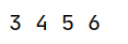
# 查一下这些属性在数据集的第几列
col_names = "total_rooms", "total_bedrooms", "population", "households"
rooms_ix, bedrooms_ix, population_ix, households_ix = [
    housing.columns.get_loc(c) for c in col_names]
print(rooms_ix, bedrooms_ix, population_ix, households_ix)
# 自定义一个转换器,用来添加组合后的属性
from sklearn.base import BaseEstimator, TransformerMixin

rooms_ix, bedrooms_ix, population_ix, households_ix = 3, 4, 5, 6


class CombinedAttributesAdder(BaseEstimator, TransformerMixin):
    def __init__(self, add_bedrooms_per_room=True):
        # 设置add_bedrooms_per_room超参数有助于知晓添加这个属性是否有助于机器学习算法
        self.add_bedrooms_per_room = add_bedrooms_per_room

    def fit(self, X, y=None):
        return self

    def transform(self, X):
        rooms_per_household = X[:, rooms_ix] / X[:, households_ix]
        population_per_household = X[:, population_ix] / X[:, households_ix]
        if self.add_bedrooms_per_room:
            bedrooms_per_room = X[:, bedrooms_ix] / X[:, rooms_ix]
            return np.c_[X, rooms_per_household, population_per_household,
                         bedrooms_per_room]
        else:
            return np.c_[X, rooms_per_household, population_per_household]


# 使用这个转换器
attr_adder = CombinedAttributesAdder(add_bedrooms_per_room=False)# 这里选择不添加add_bedrooms_per_room属性
housing_extra_attribs = attr_adder.transform(housing.values)

# 新添加的属性没有列明,为他们加上列明
housing_extra_attribs = pd.DataFrame(
    housing_extra_attribs,
    columns=list(housing.columns) + ["rooms_per_household", "population_per_household"],
    index=housing.index)
print(housing_extra_attribs.head())

# 将上述对数据的操作写成转换流水线
from sklearn.pipeline import Pipeline
from sklearn.preprocessing import StandardScaler

num_pipeline = Pipeline([
    ('imputer', SimpleImputer(strategy="median")),  # 填充空值
    ('attribs_adder', CombinedAttributesAdder()),  # 添加组合属性
    ('std_scaler', StandardScaler()),  # 数值标准化
])
housing_num_tr = num_pipeline.fit_transform(housing_num)
print(housing_num_tr)

# 将所有转换都应用到房屋数据
from sklearn.compose import ColumnTransformer

num_attribs = list(housing_num)  # 数值列
cat_attribs = ["ocean_proximity"]  # 文本列

full_pipeline = ColumnTransformer([
    ("num", num_pipeline, num_attribs),  # 数值列转换
    ("cat", OneHotEncoder(), cat_attribs),  # 文本列转换
])

housing_prepared = full_pipeline.fit_transform(housing)
print(housing_prepared)  # 打印全部都处理好的数据
print(housing_prepared.shape)

# 训练一个线性回归模型
from sklearn.linear_model import LinearRegression
lin_reg = LinearRegression()
lin_reg.fit(housing_prepared, housing_labels)
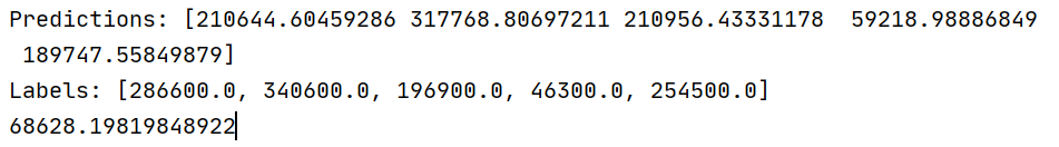
# 用几个数据来看看效果
some_data = housing.iloc[:5]
some_labels = housing_labels.iloc[:5]
some_data_prepared = full_pipeline.transform(some_data)
print("Predictions:", lin_reg.predict(some_data_prepared))
print("Labels:", list(some_labels))
# 计算一下拟合的均方根误差(RMSE)
from sklearn.metrics import mean_squared_error
housing_predictions = lin_reg.predict(housing_prepared)
lin_mse = mean_squared_error(housing_labels, housing_predictions)
lin_rmse = np.sqrt(lin_mse)
# 或者直接使用 lin_rmse = mean_squared_error(housing_labels, housing_predictions,squared=False)
print(lin_rmse) # 欠拟合
# 平均绝对误差
# from sklearn.metrics import mean_absolute_error
# lin_mae = mean_absolute_error(housing_labels, housing_predictions)
# print(lin_mae) # 49439.89599001896
# 决策树模型可以在数据中找到复杂的非线性关系
from sklearn.tree import DecisionTreeRegressor

tree_reg = DecisionTreeRegressor(random_state=42)
tree_reg.fit(housing_prepared, housing_labels)

housing_predictions = tree_reg.predict(housing_prepared)
tree_mse = mean_squared_error(housing_labels, housing_predictions)
tree_rmse = np.sqrt(tree_mse)
print(tree_rmse)  # 过拟合

# K-折交叉验证功能评估决策树模型
from sklearn.model_selection import cross_val_score

scores = cross_val_score(tree_reg, housing_prepared, housing_labels,
                         scoring="neg_mean_squared_error", cv=10)
tree_rmse_scores = np.sqrt(-scores)


# 查看评估结果
def display_scores(scores):
    print("Scores:", scores)
    print("Mean:", scores.mean())
    print("Standard deviation:", scores.std())


print(display_scores(tree_rmse_scores))

# K-折交叉验证功能评估线性回归模型
lin_scores = cross_val_score(lin_reg, housing_prepared, housing_labels,
                             scoring="neg_mean_squared_error", cv=10)
lin_rmse_scores = np.sqrt(-lin_scores)
print(display_scores(lin_rmse_scores))

# 随机森林模型
from sklearn.ensemble import RandomForestRegressor

forest_reg = RandomForestRegressor(n_estimators=100, random_state=42)  # n_estimators:子模型的数量
forest_reg.fit(housing_prepared, housing_labels)
# 整个训练集的均方根误差
housing_predictions = forest_reg.predict(housing_prepared)
forest_mse = mean_squared_error(housing_labels, housing_predictions)
forest_rmse = np.sqrt(forest_mse)
print(forest_rmse)  # 18603.515021376355
# K-折交叉验证功能评估随机森林模型
forest_scores = cross_val_score(forest_reg, housing_prepared, housing_labels,
                                scoring="neg_mean_squared_error", cv=10)
forest_rmse_scores = np.sqrt(-forest_scores)
print(display_scores(forest_rmse_scores))

# 用describe()查看线性回归模型评估分数的详情
# scores = cross_val_score(lin_reg, housing_prepared, housing_labels, scoring="neg_mean_squared_error", cv=10)
# print(pd.Series(np.sqrt(-scores)).describe())
'''
count       10.000000
mean     69052.461363
std       2879.437224
min      64969.630564
25%      67136.363758
50%      68156.372635
75%      70982.369487
max      74739.570526
dtype: float64
'''
# from sklearn.svm import SVR
#
# svm_reg = SVR(kernel="linear")  # 支持向量线性回归
# svm_reg.fit(housing_prepared, housing_labels)
# housing_predictions = svm_reg.predict(housing_prepared)
# svm_mse = mean_squared_error(housing_labels, housing_predictions)
# svm_rmse = np.sqrt(svm_mse)
# print(svm_rmse)  # 111094.6308539982
# 网格搜索,为了寻找最佳的超参数组合
from sklearn.model_selection import GridSearchCV

# 要搜索的值
param_grid = [
    {'n_estimators': [3, 10, 30], 'max_features': [2, 4, 6, 8]},
    {'bootstrap': [False], 'n_estimators': [3, 10], 'max_features': [2, 3, 4]},
]

forest_reg = RandomForestRegressor(random_state=42)  # 随机森林模型
# 每个模型进行5次训练, 一共进行 (12+6)*5=90 次训练
grid_search = GridSearchCV(forest_reg, param_grid, cv=5,
                           scoring='neg_mean_squared_error',
                           return_train_score=True)
grid_search.fit(housing_prepared, housing_labels)

# 打印最佳的参数组合
print(grid_search.best_params_)
# 打印所有模型的评估结果
cvres = grid_search.cv_results_
for mean_score, params in zip(cvres["mean_test_score"], cvres["params"]):
    print(np.sqrt(-mean_score), params)
# print(pd.DataFrame(grid_search.cv_results_))  # 打印所有模型的评估结果表格


# 随机搜索最佳的超参数组合
from sklearn.model_selection import RandomizedSearchCV
from scipy.stats import randint

param_distribs = {
    'n_estimators': randint(low=1, high=200),
    'max_features': randint(low=1, high=8),
}

forest_reg = RandomForestRegressor(random_state=42)
# n_iter=10是迭代次数
rnd_search = RandomizedSearchCV(forest_reg, param_distributions=param_distribs,
                                n_iter=10, cv=5, scoring='neg_mean_squared_error', random_state=42)
rnd_search.fit(housing_prepared, housing_labels)
print(rnd_search.best_params_)
cvres = rnd_search.cv_results_
for mean_score, params in zip(cvres["mean_test_score"], cvres["params"]):
    print(np.sqrt(-mean_score), params)

# 指出每个属性的相对重要程度(网格搜索的结果)
feature_importances = grid_search.best_estimator_.feature_importances_
print(feature_importances)

# 将这些重要性分数显示在对应的属性名称旁边
extra_attribs = ["rooms_per_hhold", "pop_per_hhold", "bedrooms_per_room"]  # 新组合属性的属性名称
cat_encoder = full_pipeline.named_transformers_["cat"]  # 对文本列进行独热编码
cat_one_hot_attribs = list(cat_encoder.categories_[0])  # 获取文本属性的类别列表
attributes = num_attribs + extra_attribs + cat_one_hot_attribs  # 所有属性的名称列表
print(sorted(zip(feature_importances, attributes), reverse=True))

# 运用测试集评估最终系统
final_model = grid_search.best_estimator_  # 运用网格搜索的最佳参数训练出的随机森林模型
# 测试集
X_test = strat_test_set.drop("median_house_value", axis=1)
y_test = strat_test_set["median_house_value"].copy()
# 处理测试集数据
X_test_prepared = full_pipeline.transform(X_test)
# 预测
final_predictions = final_model.predict(X_test_prepared)
# 均方根误差
final_mse = mean_squared_error(y_test, final_predictions)
final_rmse = np.sqrt(final_mse)  #
print(final_rmse)  # 47730.22690385927

# 95%置信区间
from scipy import stats

confidence = 0.95
squared_errors = (final_predictions - y_test) ** 2
print(np.sqrt(stats.t.interval(confidence, len(squared_errors) - 1,
                               loc=squared_errors.mean(),
                               scale=stats.sem(squared_errors))))
# array([45685.10470776, 49691.25001878])
第一题:
from sklearn.model_selection import GridSearchCV

param_grid = [
        {'kernel': ['linear'], 'C': [10., 30., 100., 300., 1000., 3000., 10000., 30000.0]},
        {'kernel': ['rbf'], 'C': [1.0, 3.0, 10., 30., 100., 300., 1000.0],
         'gamma': [0.01, 0.03, 0.1, 0.3, 1.0, 3.0]},
    ]

svm_reg = SVR()
grid_search = GridSearchCV(svm_reg, param_grid, cv=5, scoring='neg_mean_squared_error', verbose=2)
grid_search.fit(housing_prepared, housing_labels)

negative_mse = grid_search.best_score_
rmse = np.sqrt(-negative_mse)
print(rmse) # 70363.84006944533

print(grid_search.best_params_)
# {'C': 30000.0, 'kernel': 'linear'}

第二题:
from sklearn.model_selection import RandomizedSearchCV
from scipy.stats import expon, reciprocal
# Note: gamma is ignored when kernel is "linear"
param_distribs = {
        'kernel': ['linear', 'rbf'],
        'C': reciprocal(20, 200000),
        'gamma': expon(scale=1.0),
    }

svm_reg = SVR()
rnd_search = RandomizedSearchCV(svm_reg, param_distributions=param_distribs,
                                n_iter=50, cv=5, scoring='neg_mean_squared_error',
                                verbose=2, random_state=42)
rnd_search.fit(housing_prepared, housing_labels)

negative_mse = rnd_search.best_score_
rmse = np.sqrt(-negative_mse)
print(rmse)# 54767.960710084146

print(rnd_search.best_params_)
# {'C': 157055.10989448498, 'gamma': 0.26497040005002437, 'kernel': 'rbf'}


 428
428


 被折叠的 条评论
为什么被折叠?
被折叠的 条评论
为什么被折叠?
 到【灌水乐园】发言


