


 超级会员免费看
 本文详述使用LAMMPS进行热导率计算的五种方法,包括平衡态的GK法和非平衡态的NEMD/RNEMD(速度重标法、局部热浴法、动量交换法)。文章提供动态group设置、脚本获取、后处理分析和结果对比,适用于不同工况的热导率研究。
关注 M r . m a t e r i a l , \color{Violet} \rm Mr.material\ , Mr.material , 更 \color{red}{更} 更 多 \color{blue}{多} 多 精 \color{orange}{精} 精 彩 \color{green}{彩} 彩!
主要专栏内容包括:
†《LAMMPS小技巧》:
‾
\textbf{ \underline{\dag《LAMMPS小技巧》:}}
†《LAMMPS小技巧》: 主要介绍采用分子动力学(
L
a
m
m
p
s
Lammps
Lammps)模拟相关安装教程、原理以及模拟小技巧(难度:
★
\bigstar
★)
††《LAMMPS实例教程—In文件详解》:
‾
\textbf{ \underline{\dag\dag《LAMMPS实例教程—In文件详解》:}}
††《LAMMPS实例教程—In文件详解》: 主要介绍采用分子动力学(
L
a
m
m
p
s
Lammps
Lammps)模拟相关物理过程模拟。(包含:热导率计算、定压比热容计算,难度:
★
\bigstar
★
★
\bigstar
★
★
\bigstar
★)
†††《Lammps编程技巧及后处理程序技巧》:
‾
\textbf{ \underline{\dag\dag\dag《Lammps编程技巧及后处理程序技巧》:}}
†††《Lammps编程技巧及后处理程序技巧》: 主要介绍针对分子模拟的动力学过程(轨迹文件)进行后相关的处理分析(需要一定编程能力。难度:
★
\bigstar
★
★
\bigstar
★
★
\bigstar
★
★
\bigstar
★
★
\bigstar
★)。
††††《分子动力学后处理集成函数—Matlab》:
‾
\textbf{ \underline{\dag\dag\dag\dag《分子动力学后处理集成函数—Matlab》:}}
††††《分子动力学后处理集成函数—Matlab》: 主要介绍针对后处理过程中指定函数,进行包装,方便使用者直接调用(需要一定编程能力,难度:
★
\bigstar
★
★
\bigstar
★
★
\bigstar
★
★
\bigstar
★)。
†††††《SCI论文绘图—Python绘图常用模板及技巧》:
‾
\textbf{ \underline{\dag\dag\dag\dag\dag《SCI论文绘图—Python绘图常用模板及技巧》:}}
†††††《SCI论文绘图—Python绘图常用模板及技巧》: 主要介绍针对处理后的数据可视化,并提供对应的绘图模板(需要一定编程能力,难度:
★
\bigstar
★
★
\bigstar
★
★
\bigstar
★
★
\bigstar
★)。
††††††《分子模拟—Ovito渲染案例教程》:
‾
\textbf{ \underline{\dag\dag\dag\dag\dag\dag《分子模拟—Ovito渲染案例教程》:}}
††††††《分子模拟—Ovito渲染案例教程》: 主要采用
O
v
i
t
o
\rm Ovito
Ovito软件,对
L
a
m
m
p
s
\rm Lammps
Lammps 生成的轨迹文件进行渲染(难度:
★
\bigstar
★
★
\bigstar
★)。
专栏说明(订阅后可浏览对应专栏全部博文):
‾
\color{red}{\textbf{ \underline{专栏说明(订阅后可浏览对应专栏全部博文):}}}
专栏说明(订阅后可浏览对应专栏全部博文):
注意:
\color{red} 注意:
注意:如需只订阅某个单独博文,请联系博主邮箱咨询。
l
a
m
m
p
s
_
m
a
t
e
r
i
a
l
s
@
163.
c
o
m
\rm lammps\_materials@163.com
lammps_materials@163.com
♠
\spadesuit
♠
†
\dag
† 开源后处理集成程序:请关注专栏《LAMMPS后处理——MATLAB子函数合集整理》
♠
\spadesuit
♠
†
\dag
†
†
\dag
† 需要付费定制后处理程序请邮件联系:
l
a
m
m
p
s
_
m
a
t
e
r
i
a
l
s
@
163.
c
o
m
\rm lammps\_materials@163.com
lammps_materials@163.com
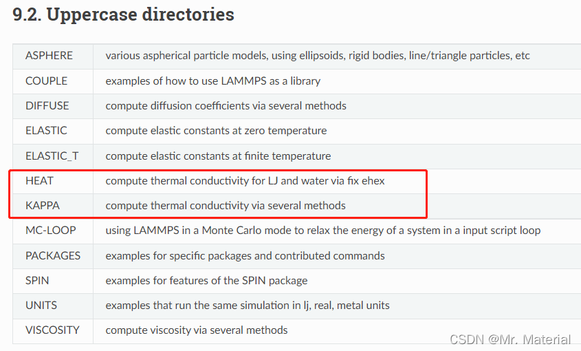
热导率计算—分子动力学
L
a
m
m
p
s
\rm Lammps
Lammps 官方案例中,提供了计算热导率的五种方法。但是按计算方法来说其实知识分为两种:平衡态分子动力学(
E
M
D
\rm EMD
EMD)、非平衡态分子动力学(
N
E
M
D
\rm NEMD
NEMD 或
R
N
E
M
D
\rm RNEMD
RNEMD)。
文章目录
- 热导率计算—分子动力学
- 注意
- 一、热传导的基本概念
- 二、大规模循环不同工况的脚本
- 三、Lammps的输出文件读取脚本—Matlab
- 四、详解五种热导率计算方法—In文件脚本
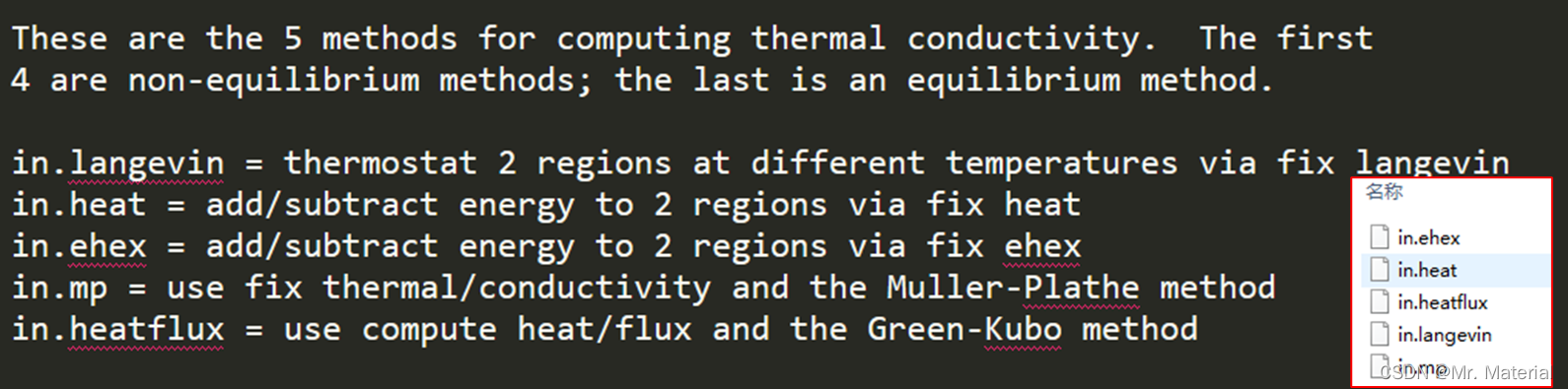
- 一、非平衡态分子动力学 ( R N E M D ) \rm (RNEMD) (RNEMD)—速度重标法 f i x e h e x \rm fix\ ehex fix ehex
- 二、非平衡态分子动力学 ( N E M D ) \rm (NEMD) (NEMD)—局部热浴法 f i x L a n g v e i n \rm fix \ Langvein fix Langvein
- 三、非平衡态分子动力学 ( R N E M D ) \rm (RNEMD) (RNEMD)—动量交换法 ( f i x t h e r m a l / c o n d u c t i v i t y ) \rm (fix\ thermal/conductivity) (fix thermal/conductivity)
- 四、非平衡态分子动力学 ( R N E M D ) \rm (RNEMD) (RNEMD)—速度重标法 ( f i x h e a t ) \rm (fix\ heat) (fix heat)
- 五、平衡态分子动力学 ( E M D ) \rm (EMD) (EMD)— G K 法 \rm GK法 GK法
- 六、五种方法结果对比
注意
1. 动态 g r o u p \rm group group 设置
针对于流体体系, 热源和热汇需要设置为动态 g r o u p \rm group group。
region            left_heat_flux   block  ${1_lattice_unit}  ${10_lattice_unit}  INF INF INF INF  units box
region            right_heat_flux  block  ${11_lattice_unit} ${all_lattice_unit} INF INF INF INF  units box

group             left_heat_flux  dynamic all region left_heat_flux  every 1

group             right_heat_flux dynamic all region right_heat_flux every 1
2. 代码说明
以固态
60
K
\rm 60\ K
60 K 下的
A
r
g
o
n
\rm Argon
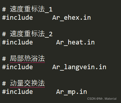
Argon 为例进行测试,脚本分为两个:
R
u
n
.
i
n
\rm Run.in
Run.in,以及几种不同方法。
运行
r
u
n
.
i
n
\rm run.in
run.in 在循环脚本中打开对应的方法即可。
3. 代码获取
(1) 全部
i
n
in
in 文件已经开源在博客,可以直接复制;
(2)
P
y
t
h
o
n
Python
Python 绘图脚本以及
I
n
In
In 文件需要打包文件请下载:
链接:请点击
6xvm
一、热传导的基本概念
1、平衡态和非平衡定态
非平衡定态
\color{red}非平衡定态
非平衡定态
体系初一环境不变的情况下,经过一定时间后,体系必将达到一个宏观上不随时间变化的状态,尽管还不一定是平衡态,但是体系将长久地保持这一状态,这样的状态称为非平衡定态,简称定态或者稳态(
s
t
a
t
i
o
n
a
r
y
s
t
a
t
e
\rm stationary\ state
stationary state).
这里环境不变的状态指的恒定外场,不变的体系体积等。当处于稳定热传导过程中,体系在宏观上属于定态,不属于平衡态,因为有热流的存在。
平衡态 \color{red}平衡态 平衡态
若处于定态的体系,同时它的环境的宏观状态也不变,则这个体系成为平衡态。
当体系从非平衡态到平衡态时,描述体系宏观状态所需的宏观参量个数达到最小。
2、热传导
首先,我们先看看传热学是如何定义热传导的。
物体各部分之间不发生相对位移时,依靠分子、原子及自由电子等微观粒子的热运动而产生的热能传递,成为热传导。(
h
e
a
t
c
o
n
d
u
c
t
i
o
n
heat\ conduction
heat conduction)下文中简称:热导。
热导现象,例如,温度较高的物体,把热量传递给与直接触的温度较低的另一固体。
热导现象的规律被总结傅里叶定律(
F
o
u
r
i
e
r
\rm Fourier
Fourier)
简单地说,对于一个一维导热问题,任意一个厚度为 d x dx dx 的单元来说。单位时间内通过该层的导热热量,与温度变化率以及平板面积 ( A A A) 成正比,即:单位时间穿过单位面积的热量,在数量上正比于温度梯度。
ϕ = − λ \phi =-\color{red}{\lambda} ϕ=−λ A d T d x A\frac{dT}{dx} AdxdT
这里的比例系数 λ \color{red}{\lambda} λ 即为导热系数。 T h e r m a l c o n d u c t i v i t y \rm Thermal\ conductivity Thermal conductivity.
显然,从上面的公式可以看出, λ \color{red}{\lambda} λ 越大代表热量越容易被输运。相同的,由于温度的不均匀性引起的能量运输称为热导现象,其运输系数称为 热导率 \rm \color{red}热导率 热导率。由于速度的不均匀性引起的动量运输,称之为黏性现象;由于体系粒子数密度的不均匀性引起的质量运输,称为扩散现象。
那么如何去计算这个热量的“运输系数”呢?这里就涉及到了,平衡态方法和非平衡态的方法。
关于这里“平衡态方法和非平衡态”的定义请参考博文《LAMMPS非平衡分子动力学 (NEMD) 纳米线热导率教程—一个代码循环计算不同温度和尺寸》
其他相关参考:
1. 《Lammps之MP方法粘度计算(包含in文件)》
2. 《轨迹分析—Matlab计算均方位移》
二、大规模循环不同工况的脚本
这里只展示代码,相关博文请参考《Lammps如何大规模循环计算?一个脚本循环不同工况》
#------------------------------------------------#
#      Author_Email: lammps_materials@163.com    #
#------------------------------------------------#
###################
# initial setting #
###################
#---------------------------------------------------------------------------#
#---------------------------------------------------------------------------#
# loop make all_file
echo   screen
print        " ------------------------------------------------"
print        " -----------------NOW making files---------------"
print        " ------------------------------------------------"
label  out_makefile
    variable     number_out loop 1
    variable     file_name_out index  60
    shell        mkdir ${file_name_out}
    shell        cp Ar_ehex.in  ${file_name_out}
    shell        cd ${file_name_out}

    # loop make in_file

        label        in_makefile

        variable     number_in loop 1
        variable     file_name_in index 10
        shell        mkdir ${file_name_in}

        shell        cp Ar_ehex.in ${file_name_in}

        next         number_in
        next         file_name_in

        jump         Ar_ehex.in  in_makefile
    clear
    # loop make in_file
    shell        cd ..
    next         number_out
    next         file_name_out

jump         Ar_ehex.in  out_makefile
clear
print        " ------------------------------------------"
print        " ------------------Finish!-----------------"
print        " ------------------------------------------"
# loop make all_file
#---------------------------------------------------------------------------#
#---------------------------------------------------------------------------#

label        calculation_in_outfile
variable     loop_number_out loop 1
# water fraction
variable     loop_file_out_name index 60
shell        cd ${loop_file_out_name}
log          ${loop_file_out_name}.log
#---------------------------------------------------------------------------#
label        calculation_in_infile
variable     loop_number_in loop 1
variable     loop_file_in_name index  10

shell        cd ${loop_file_in_name}
log          ${loop_file_in_name}.log
#---------------------------------------------------------------------------#
print        " --------------------------------------------------------------------"
print        " ----------Now the temperature is ${loop_file_out_name}-----------"
print        " ------Now lattice replicate number  is ${loop_file_in_name}------"
print        " --------------------------------------------------------------------"
#---------------------------------------------------------------------------#


include     Ar_ehex.in


#--------------------------------------------------------------#
shell        cd ..
clear
next         loop_file_in_name
jump         Ar_ehex.in calculation_in_infile
#---------------------------------------------------------------------------#
shell        cd ..
clear

next         loop_file_out_name
jump         Ar_ehex.in calculation_in_outfile
#---------------------------------------------------------------------------#
三、Lammps的输出文件读取脚本—Matlab
clc;clear;

file  = "all.temp";
%--------------------------------------------------%
num_blocks  = 20; % 体系分为20个块,这里是bin数量
num_outputs = 100;% 采样100,也就是100个温度曲线
%--------------------------------------------------%

[Chunk Coord1 Ncount v_all_temp] ...
    = textread(file, '%n%n%n%n', 'headerlines', 3, 'emptyvalue', 0);

temp = [Chunk Coord1 Ncount v_all_temp]; nall = length(temp) / (num_blocks+1);
 clear Chunk Coord1 Ncount v_all_temp;
%--------------------------------------------------%
for i =1:nall
    temp((i-1)*num_blocks+1,:)=[];
end
temp = reshape(temp(:, end), num_blocks, num_outputs);

%这里需要对温度曲线进行平均
new_temp = ave_variable(1,20,temp(:,:));
temp_all = sum(temp,2)./num_outputs;
四、详解五种热导率计算方法—In文件脚本
这里以
60
K
60K
60K
A
r
Ar
Ar的热导率为例进行对比。
非平衡分子动力学
(
N
E
M
D
)
\rm (NEMD)
(NEMD) 这里指的是通过控制温度,即施加已知温度大小的温差,计算热流。相同的
R
N
E
M
D
\rm RNEMD
RNEMD 指的是通过指定热流,计算温度梯度。
因此,采用
F
i
x
e
h
e
x
\rm Fix\ ehex
Fix ehex、
m
p
\rm mp
mp 方法的为
R
N
E
M
D
RNEMD
RNEMD;采用
F
i
x
L
a
n
g
v
e
i
n
Fix\ Langvein
Fix Langvein施加温度梯度,计算热流的为
N
E
M
D
\rm NEMD
NEMD。
一、非平衡态分子动力学 ( R N E M D ) \rm (RNEMD) (RNEMD)—速度重标法 f i x e h e x \rm fix\ ehex fix ehex
关于这个fix ehex,这个命令针对fix heat 命令的能量漂移问题,进行了修正。一些比较老的教程中可能还采用的fix heat。
核心命令 \color{red}核心命令 核心命令
fix               NVE   all nve
fix               HEAT  all ehex 1  ${POWER} region heat
fix               COLD  all ehex 1 -${POWER} region cold
clear

echo              screen
units             metal
dimension           3
boundary          p p p
atom_style        full
#----------------------------------------------------------#
variable          TS        equal 0.01                    ### ${TS} timestep
variable          Tdamp     equal 100*${TS}               ### ${Tdamp} Tdamp
variable          Pdamp     equal 1000*${TS}              ### ${Tdamp} Tdamp
variable          T         equal ${loop_file_out_name}   ### ${T} initial temperature
variable        POWER       equal 0.08
timestep         ${TS}
#----------------------------------------------------------#
#  unit cell
#----------------------------------------------------------#

variable          x_length  equal   ${loop_file_in_name}

variable          half_x    equal   ${x_length}*0.5

variable          lattice_unit      equal 5.4*2

variable          x_length    equal ${lattice_unit}*${x_length}
variable          y_length    equal ${lattice_unit}*5
variable          z_length    equal ${lattice_unit}*5

region            box block 0 ${x_length} &
                            0 ${y_length} &
                            0 ${z_length} units box
create_box        1 box
lattice           fcc 5.4
create_atoms       1 box
#----------------------------------------------------------#
variable          materials_length   equal (${half_x}-1)*${lattice_unit}

print             "=========================================="
print             "=========================================="
print             "The material length is ${materials_length}"
print             "=========================================="
print             "=========================================="
#----------------------------------------------------------#
###################
#  group setting  #
###################
#----------------------------------------------------------#
# setting mass
mass              1 40  # mass for Ar

group             Ar    type 1

velocity          all create ${T} 12345 loop local         #
#----------------------------------------------------------#
minimize          1.0e-5 1.0e-7 1000 10000
minimize          1.0e-5 1.0e-7 1000 10000
minimize          1.0e-5 1.0e-7 1000 10000

write_data        system.data
#----------------------------------------------------------#
#                     pair interaction                     #
#----------------------------------------------------------#

pair_style        lj/cut   10
pair_coeff        * *      1.032e-2 3.405

neighbor          0.5 bin
neigh_modify      every 5 delay 0 check no
#----------------------------------------------------------#

thermo            1000
#----------------------------------------------------------#
###################
#    run 1        #
###################

# loop relax system 500 ps
#----------------------------------------------------------------------#
variable         50_ps equal 50/${TS}
variable         500_ps equal 500/${TS}

variable         loop_all_num  equal 10
variable         relax_system  loop ${loop_all_num}
label            loop

fix              NVT   all   nvt temp ${T} ${T} ${Tdamp}

run              ${50_ps}

unfix            NVT
minimize         1.0e-5 1.0e-7 1000 10000
minimize         1.0e-5 1.0e-7 1000 10000

next             relax_system
jump             SELF loop

fix              NVT   all   nvt temp ${T} ${T} ${Tdamp}

run              ${500_ps}

unfix            NVT
#------------------------------------------------------------------------#
#------------------------------------------------------------------------#
#                       heat region define
#------------------------------------------------------------------------#
#
#   1    2  3  4  5  6  7  8  9  10    11   12 13 14 15 16 17 18 19 20
#   ##   ## ## ## ## ## ## ## ## ##    ##   ## ## ## ## ## ## ## ## ##
#   ##   ## ## ## ## ## ## ## ## ##    ##   ## ## ## ## ## ## ## ## ##
#    ^   <------------------------>      ^  <------------------------>
#    |             9 units               |         9 units
#   hot                                cold
#------------------------------------------------------------------------#
#                   Real length = 9*units
#------------------------------------------------------------------------#

variable          1_lattice_unit     equal  1*${lattice_unit}
variable          10_lattice_unit    equal ${half_x}*${lattice_unit}
variable          11_lattice_unit    equal (${half_x}+1)*${lattice_unit}

# heat region
region            heat  block  0                  ${1_lattice_unit}  INF INF INF INF units box

# cold region
region            cold  block  ${10_lattice_unit} ${11_lattice_unit}  INF INF INF INF units box
variable          all_lattice_unit    equal  ${x_length}*${lattice_unit}

group             heat dynamic all region heat every 1

group             cold dynamic all region cold every 1

variable          heat_flux_length     equal ${10_lattice_unit}-${1_lattice_unit}
#----------------------------------------------------------#
#----------------------------------------------------------#
region            left_heat_flux   block  ${1_lattice_unit}  ${10_lattice_unit}  INF INF INF INF  units box
region            right_heat_flux  block  ${11_lattice_unit} ${all_lattice_unit} INF INF INF INF  units box

group             left_heat_flux  dynamic all region left_heat_flux  every 1

group             right_heat_flux dynamic all region right_heat_flux every 1
#----------------------------------------------------------#
variable          HOT_temp   equal ${T}+20
variable          COLD_temp  equal ${T}-20

compute          heat heat temp/region heat
compute          cold cold temp/region cold
#----------------------------------------------------------#
#                     heat process_1
#----------------------------------------------------------#
fix               NVE   all nve
fix               HEAT  all ehex 1  ${POWER} region heat
fix               COLD  all ehex 1 -${POWER} region cold
#----------------------------------------------------------#

###################
#    run 2        #
###################
thermo_style      custom step temp pe etotal press
variable          500_ps equal  500/${TS}

run               ${500_ps}

#run               10

#----------------------------------------------------------#
#                     heat process_2
#----------------------------------------------------------#
reset_timestep 0
#----------------------------------------------------------#
#                      all temp
#----------------------------------------------------------#
variable         KB equal 8.625e-5

compute          KE all ke/atom
variable         all_temp atom c_KE/${KB}/1.5
#----------------------------------------------------------#

fix               NVE   all nve
fix               HEAT  all ehex 1  ${POWER} region heat
fix               COLD  all ehex 1 -${POWER} region cold

thermo_style      custom step temp pe etotal press  c_heat c_cold

#----------------------------------------------------------#

compute          PE all  pe/atom
compute          V all  stress/atom NULL virial

#----------------------------------------------------------#
compute           J1   left_heat_flux   heat/flux KE PE V

compute           J2   right_heat_flux  heat/flux KE PE V

variable         JJ_1    equal  c_J1[1]/${heat_flux_length}

variable         JJ_2    equal  c_J2[1]/${heat_flux_length}
#----------------------------------------------------------#

variable          block_num equal 20
variable          reduced equal 1/${block_num}

compute          layers all chunk/atom bin/1d x lower ${reduced} units reduced

# output_1 heat flux
fix              heat_flux_layer all ave/time 1 1 1 &
                 v_JJ_1  v_JJ_2  file heat_flux.txt

# output_2 temperature
fix              temp1 all ave/chunk 10 10 1000 layers                     &
                 v_all_temp file all.temp

# output_3 temperature for hot/cold
fix              ave all ave/time 1000 1 1000 c_heat c_cold file temp.txt

#----------------------------------------------------------#

###################
#    run 3        #
###################

thermo           1000
variable         1ns equal 1000/${TS}

run              ${1ns}
#run              10
相关文献:P. Jund and R. Jullien, Molecular-dynamics calculation of the thermal conductivity of vitreous silica, Physical Review B 59, 13707 (1999).
1. 后处理分析以及计算结果
1
、这里的交换的能量为
0.08
e
v
/
p
s
1、这里的交换的能量为 0.08 ev/ps
1、这里的交换的能量为0.08ev/ps
EV = 0.08
2
、将单位转换为
W
2、将单位转换为 W
2、将单位转换为W
power = EV*1.6e-7
3
、计算传热截面
3、计算传热截面
3、计算传热截面
A = 54*54*1e-20
4
、计算传热截面
4、计算传热截面
4、计算传热截面
注意,热流需要除以
2
!
\color{red}注意,热流需要除以2!
注意,热流需要除以2!
Q = power/A/2
2. Python绘图
import os
def make_save_file(filepath,filename,savename):
    # filepath 存储路径; filename:创建文件夹的名字 savename:存储图片的名字
    save_path = filepath+os.sep+filename+os.sep+savename
    all_path  = filepath+os.sep+filename
    if not os.path.exists(all_path):
        os.mkdir(all_path)
    plt.savefig(save_path,dpi=300)
filepath = r"Ar热导率"
font1 = {'family': 'Times New Roman',
             'weight': 'bold',
             'size': 18,
             }
font2 = {'family': 'Times New Roman',
             'weight': 'normal',
             'size': 11,
             }

# Global setting
# ----------------------------------------------------------------------#
import matplotlib.pyplot as plt
import pandas as pd
import numpy as np
# coding:utf-8
import pylab
import matplotlib.ticker as plticker
from matplotlib.pyplot import MultipleLocator
import xlrd
import matplotlib.pyplot as plt
from matplotlib.lines import Line2D
import math
from scipy import optimize

def f_1(x, A, B):
    return A * x + B

from scipy import optimize
plt.style.use('science')
# ----------------------------------------------------------------------#
# ----------------------------------------------------------------------#
def setup(ax,x_label,y_label):
    # 边框线的线宽设置
    width = 1.5
    ax.spines['top'].set_linewidth(width)
    ax.spines['bottom'].set_linewidth(width)
    ax.spines['left'].set_linewidth(width)
    ax.spines['right'].set_linewidth(width)
    # 边框上的ticks的出现
    ax.tick_params(top='on', bottom='on', left='on', right='on', direction='in')
    # 边框上的ticks对应的lable,即数字的尺寸
    ax.tick_params(labelsize=20,pad=6)
    #ax.yaxis.set_ticks_position('right')
    ax.tick_params(which='major', width=1.50, length=6)
    ax.tick_params(which='minor', width=0.75, length=0)
    # 边框上的ticks的出现的间隔
    locx = plticker.MultipleLocator(base=108/2) # this locator puts ticks at regular intervals
    ax.xaxis.set_major_locator(locx)
    locy = plticker.MultipleLocator(base=1) # this locator puts ticks at regular intervals
    ax.yaxis.set_major_locator(locy)
    # 边框上的注释labels
    labels = ax.get_xticklabels() + ax.get_yticklabels()
    [label.set_fontname('Times New Roman') for label in labels]
    # 边框上的注释labels距离坐标轴的距离
    xAxisLable = x_label
    yAxisLable = y_label
    ax.set_xlabel(xAxisLable, font1, labelpad=5)
    ax.set_ylabel(yAxisLable, font1, labelpad=5)
# ----------------------------------------------------------------------#
# 读取excel
excel_path = r"Ar_108.xlsx"
work_sheet = xlrd.open_workbook(excel_path);

# sheet的数量
sheet_num = work_sheet.nsheets;
# 获取sheet name
sheet_name = []
for sheet in work_sheet.sheets():
    sheet_name.append(sheet.name)
# ----------------------------------------------------------------------#
# ----------------------------------------------------------------------#
for sheet_num in range(1):
    # 选取sheet
    now_sheet = work_sheet.sheets()[0]

    # sheet的行
    row = now_sheet.nrows
    # sheet的列
    ncol = now_sheet.ncols
    #----------------------------------------------------------------------#
    #----------------------------------------------------------------------#
    font1 = {'family': 'Times New Roman',
             'weight': 'bold',
             'size': 18,
             }
    font2 = {'family': 'Times New Roman',
             'weight': 'normal',
             'size': 11,
             }
    #----------------------------------------------------------------------#
    # temp
    y10        = now_sheet.col_values(0)
    y10_matrix = list(filter(None, y10[0:]))


    markersize = 10
    linewidth = 1
    markevery =1
    alpha =1
    p_1 = dict(marker='o',color = 'r',linestyle = 'none',markevery=markevery,markerfacecolor='none',
               markersize=markersize,linewidth=linewidth,alpha=alpha)

    #----------------------------------------------------------------------#

    fig, axe = plt.subplots(1, 1, figsize=(5,5))
    xxx = np.arange(20)
    length_10 =108

    # 108 162 216 270
    axe.plot(np.arange(len(y10_matrix))*np.array(length_10)/np.array(20),  y10_matrix,**p_1,label='10.8 nm')

    scale1_left  = 2
    scale1_right = 10

    scale2_left  = 12
    scale2_right = 20

    EV    = 0.08
    power = EV*1.6e-7
    A     = 54*54*1e-20
    Q     = power/A/2

    #----------------------------------------------------------------------#
    #                    10
    #----------------------------------------------------------------------#
    x_10_1        = np.arange(len(y10_matrix))*np.array(length_10)/np.array(20)
    A10_1, B10_1  = optimize.curve_fit(f_1, x_10_1[scale1_left:scale1_right], y10_matrix[scale1_left:scale1_right])[0]
    y10_1         = A10_1 * x_10_1 + B10_1
    axe.plot(x_10_1[scale1_left:scale1_right], y10_1[scale1_left:scale1_right] , "r",ls='--',lw=2,label='Linear fitting 10.8 nm')

    x_10_2        = np.arange(len(y10_matrix))*np.array(length_10)/np.array(20)
    A10_2, B10_2  = optimize.curve_fit(f_1, x_10_1[scale2_left:scale2_right], y10_matrix[scale2_left:scale2_right])[0]
    y10_2         = A10_2 * x_10_1 + B10_2
    axe.plot(x_10_2[scale2_left:scale2_right], y10_2[scale2_left:scale2_right] , "r",ls='--',lw=2)
    print('A10')
    print('the mean is:',np.mean([abs(A10_2),abs(A10_1)]),'the std is:',np.std([abs(A10_2),abs(A10_1)]))

    temp_10_1 = (np.mean([abs(A10_2),abs(A10_1)])+np.std([abs(A10_2),abs(A10_1)]))*1e10
    temp_10_2 = (np.mean([abs(A10_2),abs(A10_1)])-np.std([abs(A10_2),abs(A10_1)]))*1e10
    kappa10_1 = Q/temp_10_1;
    kappa10_2 = Q/temp_10_2;
    print('the kappa is:',np.mean([kappa10_1,kappa10_2]),'the std is:',np.std([kappa10_1,kappa10_2]))
    print('---------------------------------------------')


    axe.set_ylim(57, 63)
    axe.set_xlim(0, 108)
    setup(axe,r'Thickness\ /$\rm \AA$',r'$\rm Temperature\ /K$')

    axe.legend(loc='best', frameon=False, \
                  labelspacing=0.3)
    axe.legend(bbox_to_anchor=(1.10, 1), \
                  loc='upper left', borderaxespad=0.,fontsize='xx-large')

    #axe[1].legend(loc='best', frameon=False, labelspacing=0.3)
    #axe[1].legend(bbox_to_anchor=(1.10, 1), loc='upper left', borderaxespad=0.,fontsize='x-large')
    # ============================================================#
    filename = "Aroutput"
    savename = "60.jpg"
    make_save_file(filepath,filename,savename)
    #figureFileName = "Amorphous_overlop.pdf"
    figureFileName = "Jump_temp.pdf"

    #plt.savefig(figureFileName, dpi=300)
    #plt.xscale("log")
    #plt.yscale("log")
    # ----------------------------------------------------------------------#

plt.show()
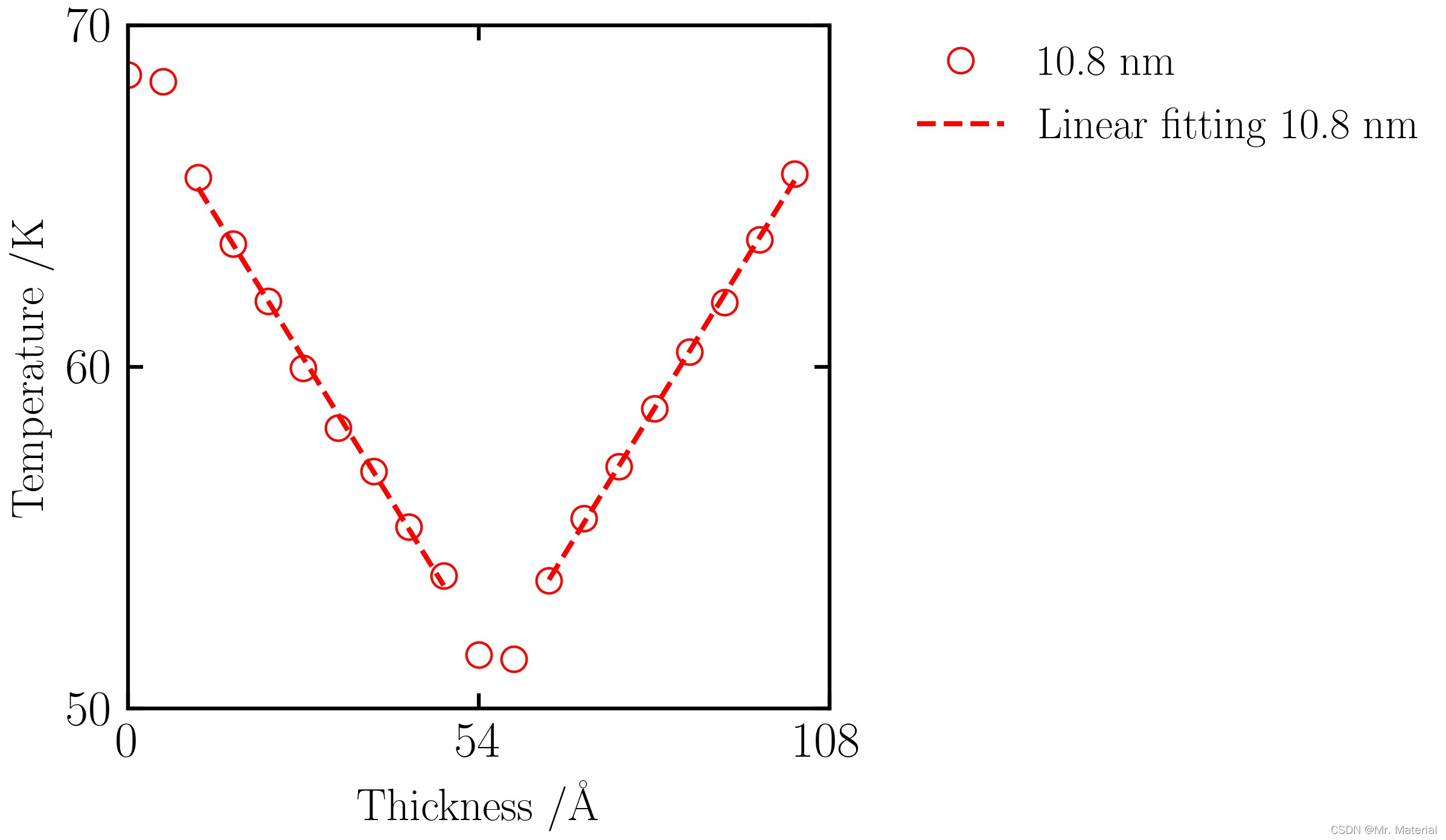
3. 报道结果
注意:这是10.8 nm,60 K下的计算结果

二、非平衡态分子动力学 ( N E M D ) \rm (NEMD) (NEMD)—局部热浴法 f i x L a n g v e i n \rm fix \ Langvein fix Langvein
核心命令 \color{red}核心命令 核心命令
fix               NVE  all     nve
fix               HEAT heat    langevin  70  70   ${Tdamp} 699483 tally  yes
fix               COLD cold    langevin  50  50   ${Tdamp} 699483 tally  yes
这里我们对热源和热汇采用 L a n g v e i n Langvein Langvein 热浴进行控温,计算热流大小。
clear

echo              screen
units             metal
dimension           3
boundary          p p p
atom_style        full
#----------------------------------------------------------#
variable          TS        equal 0.01                    ### ${TS} timestep
variable          Tdamp     equal 100*${TS}               ### ${Tdamp} Tdamp
variable          Pdamp     equal 1000*${TS}              ### ${Tdamp} Tdamp
variable          T         equal ${loop_file_out_name}   ### ${T} initial temperature
variable          POWER       equal 0.08
timestep          ${TS}
#----------------------------------------------------------#
#  unit cell
#----------------------------------------------------------#

variable          x_length  equal   ${loop_file_in_name}

variable          half_x    equal   ${x_length}*0.5

variable          lattice_unit      equal 5.4*2

variable          x_length    equal ${lattice_unit}*${x_length}
variable          y_length    equal ${lattice_unit}*5
variable          z_length    equal ${lattice_unit}*5

region            box block 0 ${x_length} &
                            0 ${y_length} &
                            0 ${z_length} units box

create_box        1 box

lattice           fcc 5.4
create_atoms      1 box
#----------------------------------------------------------#
variable          materials_length   equal (${half_x}-1)*${lattice_unit}

print             "=========================================="
print             "=========================================="
print             "The material length is ${materials_length}"
print             "=========================================="
print             "=========================================="
#----------------------------------------------------------#
###################
#  group setting  #
###################
#----------------------------------------------------------#
# setting mass
mass              1 40  # mass for Ar

group             Ar    type 1

velocity          all create ${T} 12345 loop local         #
#----------------------------------------------------------#
minimize          1.0e-5 1.0e-7 1000 10000
minimize          1.0e-5 1.0e-7 1000 10000
minimize          1.0e-5 1.0e-7 1000 10000

write_data        system.data

#----------------------------------------------------------#
#                     pair interaction                     #
#----------------------------------------------------------#

pair_style        lj/cut   10
pair_coeff        * *      1.032e-2 3.405

neighbor          0.5      bin
neigh_modify      every    5  delay 0 check no
#----------------------------------------------------------#

thermo            1000
#----------------------------------------------------------#
###################
#    run 1        #
###################

# loop relax system 500 ps
#----------------------------------------------------------------------#
variable         50_ps equal 50/${TS}
variable         500_ps equal 500/${TS}

#variable         loop_all_num  equal 1
#variable         relax_system  loop ${loop_all_num}
#label            loop

#fix              NVT   all   nvt temp ${T} ${T} ${Tdamp}

#run              ${50_ps}
#run              10

#unfix            NVT
#minimize         1.0e-5 1.0e-7 1000 10000
#minimize         1.0e-5 1.0e-7 1000 10000

#next             relax_system
#jump             SELF loop


fix              NVT   all   nvt temp ${T} ${T} ${Tdamp}

run              ${500_ps}
#run              10
unfix            NVT
#------------------------------------------------------------------------#
#------------------------------------------------------------------------#
#                       heat region define
#------------------------------------------------------------------------#
#
#   1    2  3  4  5  6  7  8  9  10    11   12 13 14 15 16 17 18 19 20
#   ##   ## ## ## ## ## ## ## ## ##    ##   ## ## ## ## ## ## ## ## ##
#   ##   ## ## ## ## ## ## ## ## ##    ##   ## ## ## ## ## ## ## ## ##
#    ^   <------------------------>      ^  <------------------------>
#    |             9 units               |         9 units
#   hot                                cold
#------------------------------------------------------------------------#
#                   Real length = 9*units
#------------------------------------------------------------------------#

variable          1_lattice_unit     equal  1*${lattice_unit}
variable          10_lattice_unit    equal ${half_x}*${lattice_unit}
variable          11_lattice_unit    equal (${half_x}+1)*${lattice_unit}

# heat region
region            heat  block  0                  ${1_lattice_unit}  INF INF INF INF units box

# cold region
region            cold  block  ${10_lattice_unit} ${11_lattice_unit}  INF INF INF INF units box
variable          all_lattice_unit    equal  ${x_length}*${lattice_unit}

group             heat                 dynamic all region heat every 1

group             cold                 dynamic all region cold every 1

variable          heat_flux_length     equal ${10_lattice_unit}-${1_lattice_unit}
#----------------------------------------------------------#
#----------------------------------------------------------#
region            left_heat_flux   block  ${1_lattice_unit}  ${10_lattice_unit}  INF INF INF INF  units box
region            right_heat_flux  block  ${11_lattice_unit} ${all_lattice_unit} INF INF INF INF  units box

group             left_heat_flux  dynamic all region left_heat_flux  every 1

group             right_heat_flux dynamic all region right_heat_flux every 1
#----------------------------------------------------------#
variable          HOT_temp   equal ${T}+20
variable          COLD_temp  equal ${T}-20

compute          heat heat temp/region heat
compute          cold cold temp/region cold
#----------------------------------------------------------#
#                     heat process_1
#----------------------------------------------------------#
fix               NVE  all     nve
fix               HEAT heat    langevin  70  70   ${Tdamp} 699483 tally  yes
fix               COLD cold    langevin  50  50   ${Tdamp} 699483 tally  yes
#----------------------------------------------------------#

###################
#    run 2        #
###################
thermo_style      custom step temp pe etotal press
variable          500_ps equal  500/${TS}

run               ${500_ps}

#run               10

#----------------------------------------------------------#
#                     heat process_2
#----------------------------------------------------------#
reset_timestep 0
#----------------------------------------------------------#
#                      all temp
#----------------------------------------------------------#
variable         KB equal 8.625e-5

compute          KE all ke/atom
variable         all_temp atom c_KE/${KB}/1.5
#----------------------------------------------------------#

fix               NVE  all     nve
fix               HEAT heat    langevin  70  70   ${Tdamp} 699483 tally  yes
fix               COLD cold    langevin  50  50   ${Tdamp} 699483 tally  yes

thermo_style      custom step temp pe etotal press  c_heat c_cold f_HEAT  f_COLD


#----------------------------------------------------------#

compute          PE all  pe/atom

#----------------------------------------------------------#

variable          block_num equal 20
variable          reduced   equal 1/${block_num}

compute          layers all chunk/atom bin/1d x lower ${reduced} units reduced

# output_1 temperature
fix              temp1 all ave/chunk 10 10 1000 layers                     &
                 v_all_temp file all.temp

# output_2 exchange energy
fix              heat_flux_layer all ave/time 10 10 100 &
                 f_HEAT  f_COLD  file heat_flux_exchange.txt

#----------------------------------------------------------#

###################
#    run 3        #
###################

thermo           1000
variable         1ns equal 1000/${TS}

run              ${1ns}
#run              10
1. 后处理分析以及计算结果
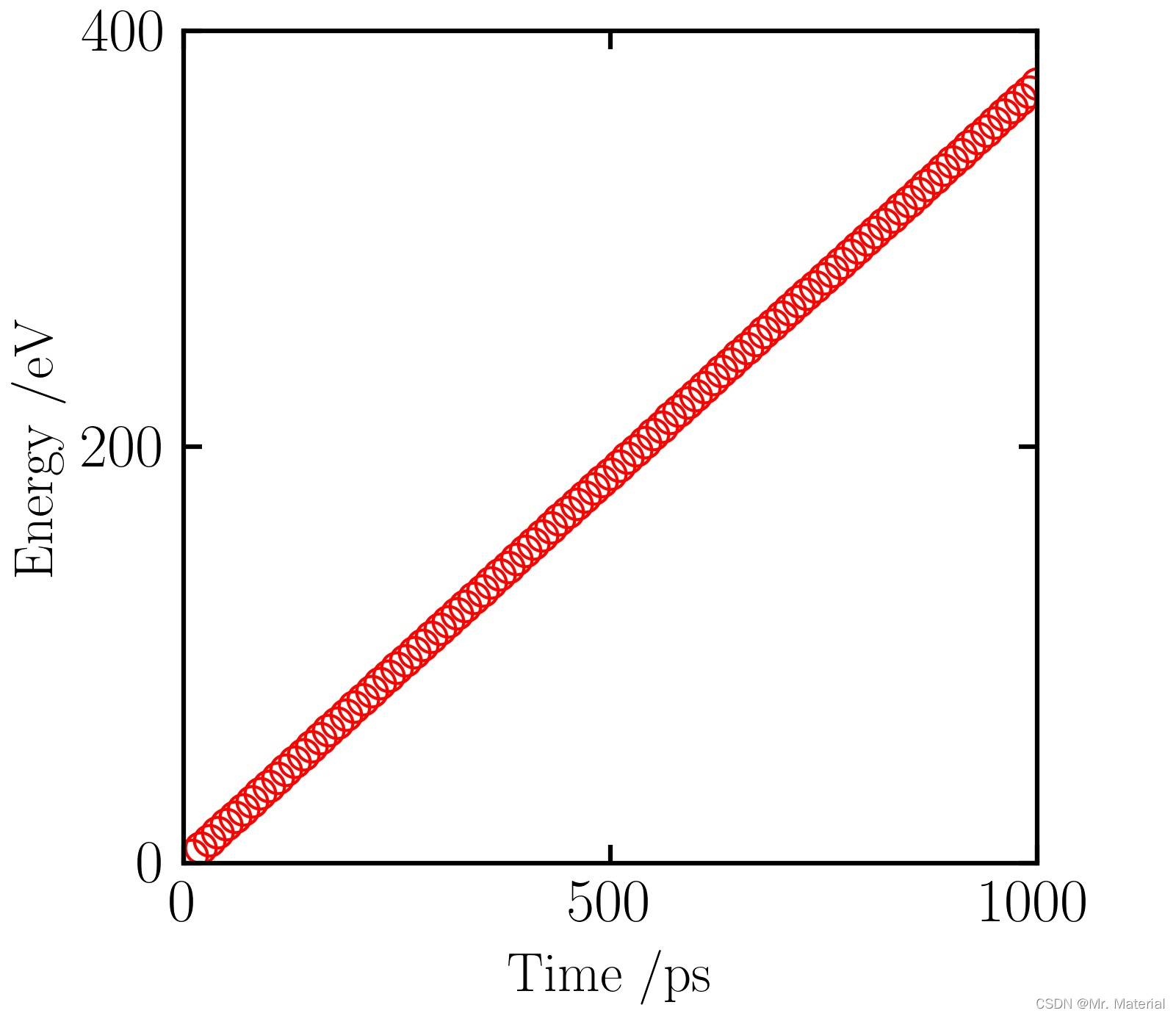
热功率计算
这里我们根据在统计热源、热汇和热浴交换的能量,计算热功率。这里我们统计了1 n s \rm ns ns,总能量为316 e V \rm eV eV,那么交换的热功率为0.3 e V / p s \rm eV/ps eV/ps.
核心命令 \color{red} 核心命令 核心命令
fix               NVE  all     nve
fix               HEAT heat    langevin  70  70   ${Tdamp} 699483 tally  yes
fix               COLD cold    langevin  50  50   ${Tdamp} 699483 tally  yes
...

# output_2 exchange energy
fix              heat_flux_layer all ave/time 10 10 100 &
                 f_HEAT  f_COLD  file heat_flux_exchange.txt
import os
def make_save_file(filepath,filename,savename):
    # filepath 存储路径; filename:创建文件夹的名字 savename:存储图片的名字
    save_path = filepath+os.sep+filename+os.sep+savename
    all_path  = filepath+os.sep+filename
    if not os.path.exists(all_path):
        os.mkdir(all_path)
    plt.savefig(save_path,dpi=300)
filepath = r"Ar热导率"
font1 = {'family': 'Times New Roman',
             'weight': 'bold',
             'size': 18,
             }
font2 = {'family': 'Times New Roman',
             'weight': 'normal',
             'size': 11,
             }

# Global setting
# ----------------------------------------------------------------------#
import matplotlib.pyplot as plt
import pandas as pd
import numpy as np
# coding:utf-8
import pylab
import matplotlib.ticker as plticker
from matplotlib.pyplot import MultipleLocator
import xlrd
import matplotlib.pyplot as plt
from matplotlib.lines import Line2D
import math
from scipy import optimize

def f_1(x, A, B):
    return A * x + B

from scipy import optimize
plt.style.use('science')
# ----------------------------------------------------------------------#
# ----------------------------------------------------------------------#
def setup(ax,x_label,y_label):
    # 边框线的线宽设置
    width = 1.5
    ax.spines['top'].set_linewidth(width)
    ax.spines['bottom'].set_linewidth(width)
    ax.spines['left'].set_linewidth(width)
    ax.spines['right'].set_linewidth(width)
    # 边框上的ticks的出现
    ax.tick_params(top='on', bottom='on', left='on', right='on', direction='in')
    # 边框上的ticks对应的lable,即数字的尺寸
    ax.tick_params(labelsize=20,pad=6)
    #ax.yaxis.set_ticks_position('right')
    ax.tick_params(which='major', width=1.50, length=6)
    ax.tick_params(which='minor', width=0.75, length=0)
    # 边框上的ticks的出现的间隔
    locx = plticker.MultipleLocator(base=500) # this locator puts ticks at regular intervals
    ax.xaxis.set_major_locator(locx)
    locy = plticker.MultipleLocator(base=320/2) # this locator puts ticks at regular intervals
    ax.yaxis.set_major_locator(locy)
    # 边框上的注释labels
    labels = ax.get_xticklabels() + ax.get_yticklabels()
    [label.set_fontname('Times New Roman') for label in labels]
    # 边框上的注释labels距离坐标轴的距离
    xAxisLable = x_label
    yAxisLable = y_label
    ax.set_xlabel(xAxisLable, font1, labelpad=5)
    ax.set_ylabel(yAxisLable, font1, labelpad=5)
# ----------------------------------------------------------------------#
# 读取excel
excel_path = r"Ar_108.xlsx"
work_sheet = xlrd.open_workbook(excel_path);

# sheet的数量
sheet_num = work_sheet.nsheets;
# 获取sheet name
sheet_name = []
for sheet in work_sheet.sheets():
    sheet_name.append(sheet.name)
# ----------------------------------------------------------------------#
# ----------------------------------------------------------------------#
for sheet_num in range(1):
    # 选取sheet
    now_sheet = work_sheet.sheets()[0]

    # sheet的行
    row = now_sheet.nrows
    # sheet的列
    ncol = now_sheet.ncols
    #----------------------------------------------------------------------#
    #----------------------------------------------------------------------#
    font1 = {'family': 'Times New Roman',
             'weight': 'bold',
             'size': 18,
             }
    font2 = {'family': 'Times New Roman',
             'weight': 'normal',
             'size': 11,
             }
    #----------------------------------------------------------------------#
    # temp
    hot        = now_sheet.col_values(2)
    hot_matrix = list(filter(None, hot[1:]))

    cold        = now_sheet.col_values(3)
    cold_matrix = list(filter(None, cold[1:]))

    markersize = 10
    linewidth = 1
    markevery =50
    alpha =1
    p_1 = dict(marker='o',color = 'r',linestyle = 'none',markevery=markevery,markerfacecolor='none',
               markersize=markersize,linewidth=linewidth,alpha=alpha)
    p_2 = dict(marker='o',color = 'b',linestyle = 'none',markevery=markevery,markerfacecolor='none',
               markersize=markersize,linewidth=linewidth,alpha=alpha)
    #----------------------------------------------------------------------#

    fig, axe = plt.subplots(1, 1, figsize=(5,5))
    xxx = np.arange(20)
    length_10 =108

    # 108 162 216 270
    axe.plot(np.arange(len(hot_matrix)),  hot_matrix,**p_1)
    axe.plot(np.arange(len(hot_matrix)),  cold_matrix,**p_2)

    axe.set_ylim(-320, 320)
    axe.set_xlim(0, 1000)
    setup(axe,r'Time\ /$\rm ps$',r'$\rm Energy\ /eV$')

    axe.legend(loc='best', frameon=False, \
                  labelspacing=0.3)
    axe.legend(bbox_to_anchor=(1.10, 1), \
                  loc='upper left', borderaxespad=0.,fontsize='xx-large')

    #axe[1].legend(loc='best', frameon=False, labelspacing=0.3)
    #axe[1].legend(bbox_to_anchor=(1.10, 1), loc='upper left', borderaxespad=0.,fontsize='x-large')
    # ============================================================#
    filename = "Aroutput"
    savename = "eV.jpg"
    make_save_file(filepath,filename,savename)
    #figureFileName = "Amorphous_overlop.pdf"
    figureFileName = "Jump_temp.pdf"

    #plt.savefig(figureFileName, dpi=300)
    #plt.xscale("log")
    #plt.yscale("log")
    # ----------------------------------------------------------------------#

plt.show()
2. 温度梯度拟合
import os
def make_save_file(filepath,filename,savename):
    # filepath 存储路径; filename:创建文件夹的名字 savename:存储图片的名字
    save_path = filepath+os.sep+filename+os.sep+savename
    all_path  = filepath+os.sep+filename
    if not os.path.exists(all_path):
        os.mkdir(all_path)
    plt.savefig(save_path,dpi=300)
filepath = r"Ar热导率"
font1 = {'family': 'Times New Roman',
             'weight': 'bold',
             'size': 18,
             }
font2 = {'family': 'Times New Roman',
             'weight': 'normal',
             'size': 11,
             }

# Global setting
# ----------------------------------------------------------------------#
import matplotlib.pyplot as plt
import pandas as pd
import numpy as np
# coding:utf-8
import pylab
import matplotlib.ticker as plticker
from matplotlib.pyplot import MultipleLocator
import xlrd
import matplotlib.pyplot as plt
from matplotlib.lines import Line2D
import math
from scipy import optimize

def f_1(x, A, B):
    return A * x + B

from scipy import optimize
plt.style.use('science')
# ----------------------------------------------------------------------#
# ----------------------------------------------------------------------#
def setup(ax,x_label,y_label):
    # 边框线的线宽设置
    width = 1.5
    ax.spines['top'].set_linewidth(width)
    ax.spines['bottom'].set_linewidth(width)
    ax.spines['left'].set_linewidth(width)
    ax.spines['right'].set_linewidth(width)
    # 边框上的ticks的出现
    ax.tick_params(top='on', bottom='on', left='on', right='on', direction='in')
    # 边框上的ticks对应的lable,即数字的尺寸
    ax.tick_params(labelsize=20,pad=6)
    #ax.yaxis.set_ticks_position('right')
    ax.tick_params(which='major', width=1.50, length=6)
    ax.tick_params(which='minor', width=0.75, length=0)
    # 边框上的ticks的出现的间隔
    locx = plticker.MultipleLocator(base=108/2) # this locator puts ticks at regular intervals
    ax.xaxis.set_major_locator(locx)
    locy = plticker.MultipleLocator(base=10) # this locator puts ticks at regular intervals
    ax.yaxis.set_major_locator(locy)
    # 边框上的注释labels
    labels = ax.get_xticklabels() + ax.get_yticklabels()
    [label.set_fontname('Times New Roman') for label in labels]
    # 边框上的注释labels距离坐标轴的距离
    xAxisLable = x_label
    yAxisLable = y_label
    ax.set_xlabel(xAxisLable, font1, labelpad=5)
    ax.set_ylabel(yAxisLable, font1, labelpad=5)
# ----------------------------------------------------------------------#
# 读取excel
excel_path = r"Ar_108.xlsx"
work_sheet = xlrd.open_workbook(excel_path);

# sheet的数量
sheet_num = work_sheet.nsheets;
# 获取sheet name
sheet_name = []
for sheet in work_sheet.sheets():
    sheet_name.append(sheet.name)
# ----------------------------------------------------------------------#
# ----------------------------------------------------------------------#
for sheet_num in range(1):
    # 选取sheet
    now_sheet = work_sheet.sheets()[0]

    # sheet的行
    row = now_sheet.nrows
    # sheet的列
    ncol = now_sheet.ncols
    #----------------------------------------------------------------------#
    #----------------------------------------------------------------------#
    font1 = {'family': 'Times New Roman',
             'weight': 'bold',
             'size': 18,
             }
    font2 = {'family': 'Times New Roman',
             'weight': 'normal',
             'size': 11,
             }
    #----------------------------------------------------------------------#
    # temp
    y10        = now_sheet.col_values(1)
    y10_matrix = list(filter(None, y10[1:]))


    markersize = 10
    linewidth = 1
    markevery =1
    alpha =1
    p_1 = dict(marker='o',color = 'r',linestyle = 'none',markevery=markevery,markerfacecolor='none',
               markersize=markersize,linewidth=linewidth,alpha=alpha)

    #----------------------------------------------------------------------#

    fig, axe = plt.subplots(1, 1, figsize=(5,5))
    xxx = np.arange(20)
    length_10 =108

    # 108 162 216 270
    axe.plot(np.arange(len(y10_matrix))*np.array(length_10)/np.array(20),  y10_matrix,**p_1,label='10.8 nm')

    scale1_left  = 2
    scale1_right = 10

    scale2_left  = 12
    scale2_right = 20

    EV    = 0.3
    power = EV*1.6e-7
    A     = 54*54*1e-20
    Q     = power/A/2

    #----------------------------------------------------------------------#
    #                    10
    #----------------------------------------------------------------------#
    x_10_1        = np.arange(len(y10_matrix))*np.array(length_10)/np.array(20)
    A10_1, B10_1  = optimize.curve_fit(f_1, x_10_1[scale1_left:scale1_right], y10_matrix[scale1_left:scale1_right])[0]
    y10_1         = A10_1 * x_10_1 + B10_1
    axe.plot(x_10_1[scale1_left:scale1_right], y10_1[scale1_left:scale1_right] , "r",ls='--',lw=2,label='Linear fitting 10.8 nm')

    x_10_2        = np.arange(len(y10_matrix))*np.array(length_10)/np.array(20)
    A10_2, B10_2  = optimize.curve_fit(f_1, x_10_1[scale2_left:scale2_right], y10_matrix[scale2_left:scale2_right])[0]
    y10_2         = A10_2 * x_10_1 + B10_2
    axe.plot(x_10_2[scale2_left:scale2_right], y10_2[scale2_left:scale2_right] , "r",ls='--',lw=2)
    print('A10')
    print('the mean is:',np.mean([abs(A10_2),abs(A10_1)]),'the std is:',np.std([abs(A10_2),abs(A10_1)]))

    temp_10_1 = (np.mean([abs(A10_2),abs(A10_1)])+np.std([abs(A10_2),abs(A10_1)]))*1e10
    temp_10_2 = (np.mean([abs(A10_2),abs(A10_1)])-np.std([abs(A10_2),abs(A10_1)]))*1e10
    kappa10_1 = Q/temp_10_1;
    kappa10_2 = Q/temp_10_2;
    print('the kappa is:',np.mean([kappa10_1,kappa10_2]),'the std is:',np.std([kappa10_1,kappa10_2]))
    print('---------------------------------------------')


    axe.set_ylim(50, 70)
    axe.set_xlim(0, 108)
    setup(axe,r'Thickness\ /$\rm \AA$',r'$\rm Temperature\ /K$')

    axe.legend(loc='best', frameon=False, \
                  labelspacing=0.3)
    axe.legend(bbox_to_anchor=(1.10, 1), \
                  loc='upper left', borderaxespad=0.,fontsize='xx-large')

    #axe[1].legend(loc='best', frameon=False, labelspacing=0.3)
    #axe[1].legend(bbox_to_anchor=(1.10, 1), loc='upper left', borderaxespad=0.,fontsize='x-large')
    # ============================================================#
    filename = "Aroutput"
    savename = "langvein.jpg"
    make_save_file(filepath,filename,savename)
    #figureFileName = "Amorphous_overlop.pdf"
    figureFileName = "Jump_temp.pdf"

    #plt.savefig(figureFileName, dpi=300)
    #plt.xscale("log")
    #plt.yscale("log")
    # ----------------------------------------------------------------------#

plt.show()
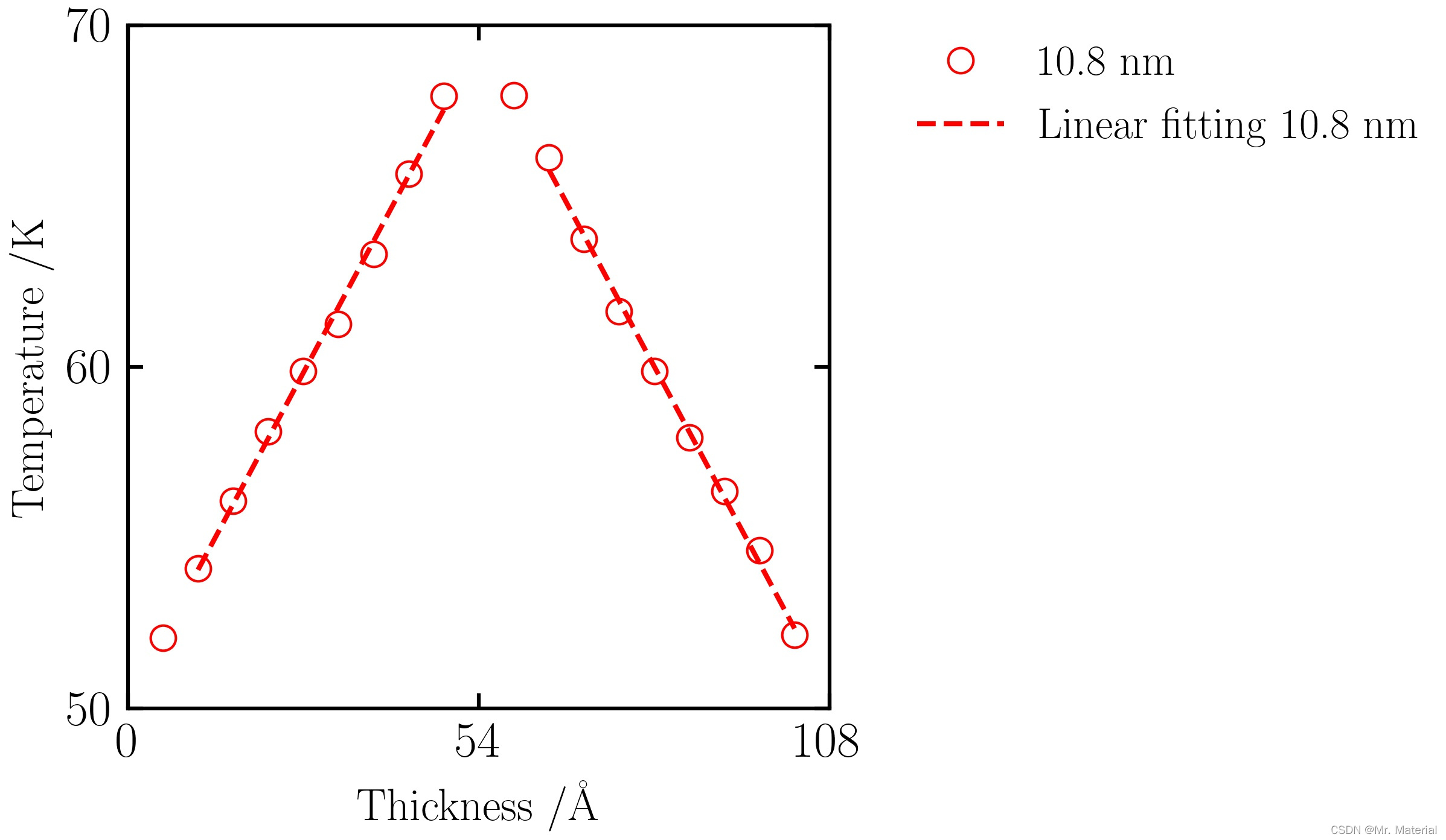
3. 报道结果

三、非平衡态分子动力学 ( R N E M D ) \rm (RNEMD) (RNEMD)—动量交换法 ( f i x t h e r m a l / c o n d u c t i v i t y ) \rm (fix\ thermal/conductivity) (fix thermal/conductivity)
核心命令:
\color{red}核心命令:
核心命令:
这里注意分块一定要是整数。
#------------------------------------------------------------------------#
#
#   1    2  3  4  5  6  7  8  9  10    11   12 13 14 15 16 17 18 19 20
#   ##   ## ## ## ## ## ## ## ## ##    ##   ## ## ## ## ## ## ## ## ##
#   ##   ## ## ## ## ## ## ## ## ##    ##   ## ## ## ## ## ## ## ## ##
#    ^   <------------------------>      ^  <------------------------>
#    |             9 units               |         9 units
#   hot                                cold
#------------------------------------------------------------------------#

fix               NVE   all nve
fix               mp    all thermal/conductivity 10 x 20
clear

echo              screen
units             metal
dimension           3
boundary          p p p
atom_style        full
#----------------------------------------------------------#
variable          TS        equal 0.01                    ### ${TS} timestep
variable          Tdamp     equal 100*${TS}               ### ${Tdamp} Tdamp
variable          Pdamp     equal 1000*${TS}              ### ${Tdamp} Tdamp
variable          T         equal ${loop_file_out_name}   ### ${T} initial temperature
variable        POWER       equal 0.08
timestep         ${TS}
#----------------------------------------------------------#
#  unit cell
#----------------------------------------------------------#

variable          x_length  equal   ${loop_file_in_name}

variable          half_x    equal   ${x_length}*0.5

variable          lattice_unit      equal 5.4*2

variable          x_length    equal ${lattice_unit}*${x_length}
variable          y_length    equal ${lattice_unit}*5
variable          z_length    equal ${lattice_unit}*5

region            box block 0 ${x_length} &
                            0 ${y_length} &
                            0 ${z_length} units box
create_box        1 box
lattice           fcc 5.4
create_atoms       1 box
#----------------------------------------------------------#
variable          materials_length   equal (${half_x}-1)*${lattice_unit}

print             "=========================================="
print             "=========================================="
print             "The material length is ${materials_length}"
print             "=========================================="
print             "=========================================="
#----------------------------------------------------------#
###################
#  group setting  #
###################
#----------------------------------------------------------#
# setting mass
mass              1 40  # mass for Ar

group             Ar    type 1

velocity          all create ${T} 12345 loop local         #
#----------------------------------------------------------#
minimize          1.0e-5 1.0e-7 1000 10000
minimize          1.0e-5 1.0e-7 1000 10000
minimize          1.0e-5 1.0e-7 1000 10000

write_data        system.data
#----------------------------------------------------------#
#                     pair interaction                     #
#----------------------------------------------------------#

pair_style        lj/cut   10
pair_coeff        * *      1.032e-2 3.405

neighbor          0.5 bin
neigh_modify      every 5 delay 0 check no
#----------------------------------------------------------#

thermo            1000
#----------------------------------------------------------#
###################
#    run 1        #
###################

# loop relax system 500 ps
#----------------------------------------------------------------------#
variable         50_ps equal 50/${TS}
variable         500_ps equal 500/${TS}

variable         loop_all_num  equal 10
variable         relax_system  loop ${loop_all_num}
label            loop

fix              NVT   all   nvt temp ${T} ${T} ${Tdamp}

run              ${50_ps}

unfix            NVT
minimize         1.0e-5 1.0e-7 1000 10000
minimize         1.0e-5 1.0e-7 1000 10000

next             relax_system
jump             SELF loop

fix              NVT   all   nvt temp ${T} ${T} ${Tdamp}

run              ${500_ps}

unfix            NVT
#------------------------------------------------------------------------#
#------------------------------------------------------------------------#
#                       heat region define
#------------------------------------------------------------------------#
#
#   1    2  3  4  5  6  7  8  9  10    11   12 13 14 15 16 17 18 19 20
#   ##   ## ## ## ## ## ## ## ## ##    ##   ## ## ## ## ## ## ## ## ##
#   ##   ## ## ## ## ## ## ## ## ##    ##   ## ## ## ## ## ## ## ## ##
#    ^   <------------------------>      ^  <------------------------>
#    |             9 units               |         9 units
#   hot                                cold
#------------------------------------------------------------------------#
#                   Real length = 9*units
#------------------------------------------------------------------------#

variable          1_lattice_unit     equal  1*${lattice_unit}
variable          10_lattice_unit    equal ${half_x}*${lattice_unit}
variable          11_lattice_unit    equal (${half_x}+1)*${lattice_unit}

# heat region
region            heat  block  0                  ${1_lattice_unit}  INF INF INF INF units box

# cold region
region            cold  block  ${10_lattice_unit} ${11_lattice_unit}  INF INF INF INF units box
variable          all_lattice_unit    equal  ${x_length}*${lattice_unit}

group             heat dynamic all region heat every 1

group             cold dynamic all region cold every 1

variable          heat_flux_length     equal ${10_lattice_unit}-${1_lattice_unit}
#----------------------------------------------------------#
#----------------------------------------------------------#
region            left_heat_flux   block  ${1_lattice_unit}  ${10_lattice_unit}  INF INF INF INF  units box
region            right_heat_flux  block  ${11_lattice_unit} ${all_lattice_unit} INF INF INF INF  units box

group             left_heat_flux  dynamic all region left_heat_flux  every 1

group             right_heat_flux dynamic all region right_heat_flux every 1
#----------------------------------------------------------#
variable          HOT_temp   equal ${T}+20
variable          COLD_temp  equal ${T}-20

compute          heat heat temp/region heat
compute          cold cold temp/region cold
#----------------------------------------------------------#
#                     heat process_1
#----------------------------------------------------------#
fix               NVE   all nve
fix               mp   all thermal/conductivity 10 x 20
#----------------------------------------------------------#

###################
#    run 2        #
###################
thermo_style      custom step temp pe etotal press
variable          500_ps equal  500/${TS}

run               ${500_ps}

#run               10

#----------------------------------------------------------#
#                     heat process_2
#----------------------------------------------------------#
reset_timestep 0
#----------------------------------------------------------#
#                      all temp
#----------------------------------------------------------#
variable         KB equal 8.625e-5

compute          KE all ke/atom
variable         all_temp atom c_KE/${KB}/1.5
#----------------------------------------------------------#

fix               NVE   all nve
fix               mp   all thermal/conductivity 10 x 20

thermo_style      custom step temp pe etotal press  c_heat c_cold

#----------------------------------------------------------#

compute          PE all  pe/atom

#----------------------------------------------------------#

variable          block_num equal 20
variable          reduced equal 1/${block_num}

compute          layers all chunk/atom bin/1d x lower ${reduced} units reduced


# output_1 temperature
fix              temp1 all ave/chunk 10 10 1000 layers                     &
                 v_all_temp file all.temp

# output_2 temperature for hot/cold
fix              ave all ave/time 10 10 1000 c_heat c_cold file temp.txt

# output_3 energy
fix              ave all ave/time 10 10 1000 f_mp file ev.txt
#----------------------------------------------------------#

###################
#    run 3        #
###################

thermo           1000
variable         1ns equal 1000/${TS}

run              ${1ns}
#run              10
1. 能量输出
2. 温度拟合
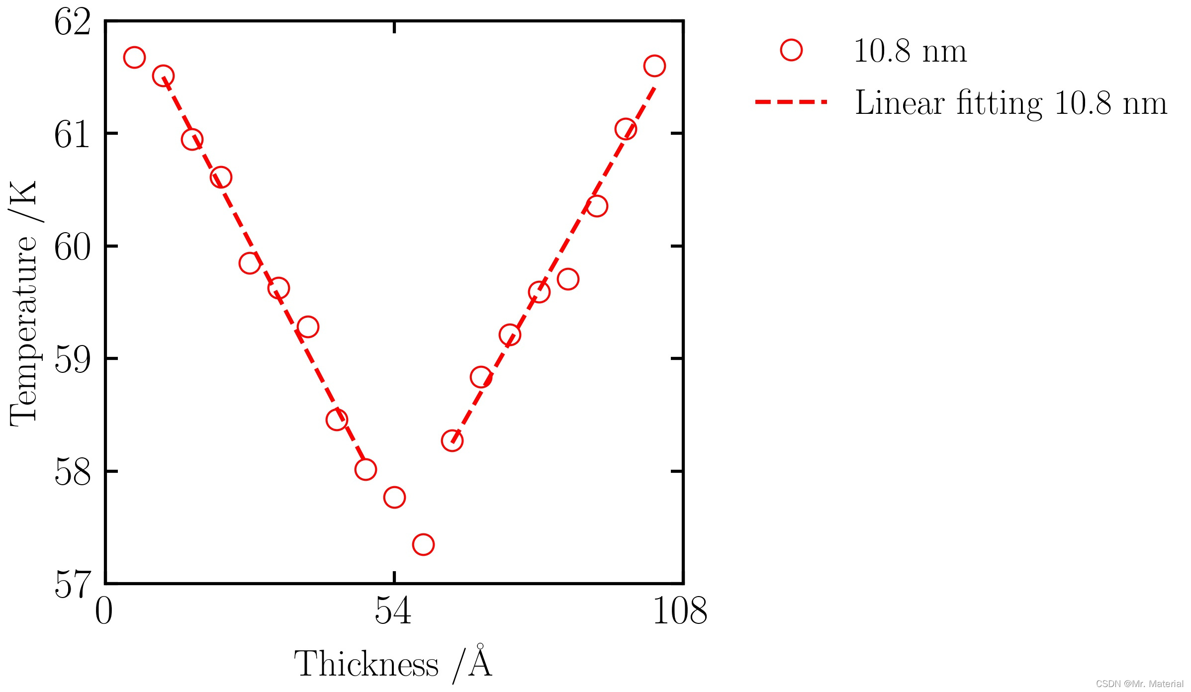
3. 报道结果

四、非平衡态分子动力学 ( R N E M D ) \rm (RNEMD) (RNEMD)—速度重标法 ( f i x h e a t ) \rm (fix\ heat) (fix heat)
核心命令: \color{red}核心命令: 核心命令:
fix               NVE   all nve
fix               HEAT  all heat 1  ${POWER} region heat
fix               COLD  all heat 1 -${POWER} region cold
这里的后处理的方法, f i x h e a t fix\ heat fix heat 和 f i x e h x fix\ ehx fix ehx 方法完全类似,这里不再赘述。
clear

echo              screen
units             metal
dimension           3
boundary          p p p
atom_style        full
#----------------------------------------------------------#
variable          TS        equal 0.01                    ### ${TS} timestep
variable          Tdamp     equal 100*${TS}               ### ${Tdamp} Tdamp
variable          Pdamp     equal 1000*${TS}              ### ${Tdamp} Tdamp
variable          T         equal ${loop_file_out_name}   ### ${T} initial temperature
variable        POWER       equal 0.08
timestep         ${TS}
#----------------------------------------------------------#
#  unit cell
#----------------------------------------------------------#

variable          x_length  equal   ${loop_file_in_name}

variable          half_x    equal   ${x_length}*0.5

variable          lattice_unit      equal 5.4*2

variable          x_length    equal ${lattice_unit}*${x_length}
variable          y_length    equal ${lattice_unit}*5
variable          z_length    equal ${lattice_unit}*5

region            box block 0 ${x_length} &
                            0 ${y_length} &
                            0 ${z_length} units box
create_box        1 box
lattice           fcc 5.4
create_atoms       1 box
#----------------------------------------------------------#
variable          materials_length   equal (${half_x}-1)*${lattice_unit}

print             "=========================================="
print             "=========================================="
print             "The material length is ${materials_length}"
print             "=========================================="
print             "=========================================="
#----------------------------------------------------------#
###################
#  group setting  #
###################
#----------------------------------------------------------#
# setting mass
mass              1 40  # mass for Ar

group             Ar    type 1

velocity          all create ${T} 12345 loop local         #
#----------------------------------------------------------#
minimize          1.0e-5 1.0e-7 1000 10000
minimize          1.0e-5 1.0e-7 1000 10000
minimize          1.0e-5 1.0e-7 1000 10000

write_data        system.data
#----------------------------------------------------------#
#                     pair interaction                     #
#----------------------------------------------------------#

pair_style        lj/cut   10
pair_coeff        * *      1.032e-2 3.405

neighbor          0.5 bin
neigh_modify      every 5 delay 0 check no
#----------------------------------------------------------#

thermo            1000
#----------------------------------------------------------#
###################
#    run 1        #
###################

# loop relax system 500 ps
#----------------------------------------------------------------------#
variable         50_ps equal 50/${TS}
variable         500_ps equal 500/${TS}

variable         loop_all_num  equal 10
variable         relax_system  loop ${loop_all_num}
label            loop

fix              NVT   all   nvt temp ${T} ${T} ${Tdamp}

run              ${50_ps}

unfix            NVT
minimize         1.0e-5 1.0e-7 1000 10000
minimize         1.0e-5 1.0e-7 1000 10000

next             relax_system
jump             SELF loop

fix              NVT   all   nvt temp ${T} ${T} ${Tdamp}

run              ${500_ps}

unfix            NVT
#------------------------------------------------------------------------#
#------------------------------------------------------------------------#
#                       heat region define
#------------------------------------------------------------------------#
#
#   1    2  3  4  5  6  7  8  9  10    11   12 13 14 15 16 17 18 19 20
#   ##   ## ## ## ## ## ## ## ## ##    ##   ## ## ## ## ## ## ## ## ##
#   ##   ## ## ## ## ## ## ## ## ##    ##   ## ## ## ## ## ## ## ## ##
#    ^   <------------------------>      ^  <------------------------>
#    |             9 units               |         9 units
#   hot                                cold
#------------------------------------------------------------------------#
#                   Real length = 9*units
#------------------------------------------------------------------------#

variable          1_lattice_unit     equal  1*${lattice_unit}
variable          10_lattice_unit    equal ${half_x}*${lattice_unit}
variable          11_lattice_unit    equal (${half_x}+1)*${lattice_unit}

# heat region
region            heat  block  0                  ${1_lattice_unit}  INF INF INF INF units box

# cold region
region            cold  block  ${10_lattice_unit} ${11_lattice_unit}  INF INF INF INF units box
variable          all_lattice_unit    equal  ${x_length}*${lattice_unit}

group             heat dynamic all region heat every 1

group             cold dynamic all region cold every 1

variable          heat_flux_length     equal ${10_lattice_unit}-${1_lattice_unit}
#----------------------------------------------------------#
#----------------------------------------------------------#
region            left_heat_flux   block  ${1_lattice_unit}  ${10_lattice_unit}  INF INF INF INF  units box
region            right_heat_flux  block  ${11_lattice_unit} ${all_lattice_unit} INF INF INF INF  units box

group             left_heat_flux  dynamic all region left_heat_flux  every 1

group             right_heat_flux dynamic all region right_heat_flux every 1
#----------------------------------------------------------#
variable          HOT_temp   equal ${T}+20
variable          COLD_temp  equal ${T}-20

compute          heat heat temp/region heat
compute          cold cold temp/region cold
#----------------------------------------------------------#
#                     heat process_1
#----------------------------------------------------------#
fix               NVE   all nve
fix               HEAT  all heat 1  ${POWER} region heat
fix               COLD  all heat 1 -${POWER} region cold
#----------------------------------------------------------#

###################
#    run 2        #
###################
thermo_style      custom step temp pe etotal press
variable          500_ps equal  500/${TS}

run               ${500_ps}

#run               10

#----------------------------------------------------------#
#                     heat process_2
#----------------------------------------------------------#
reset_timestep 0
#----------------------------------------------------------#
#                      all temp
#----------------------------------------------------------#
variable         KB equal 8.625e-5

compute          KE all ke/atom
variable         all_temp atom c_KE/${KB}/1.5
#----------------------------------------------------------#

fix               NVE   all nve
fix               HEAT  all heat 1  ${POWER} region heat
fix               COLD  all heat 1 -${POWER} region cold

thermo_style      custom step temp pe etotal press  c_heat c_cold

#----------------------------------------------------------#

compute          PE all  pe/atom
compute          V all  stress/atom NULL virial

#----------------------------------------------------------#
compute           J1   left_heat_flux   heat/flux KE PE V

compute           J2   right_heat_flux  heat/flux KE PE V

variable         JJ_1    equal  c_J1[1]/${heat_flux_length}

variable         JJ_2    equal  c_J2[1]/${heat_flux_length}
#----------------------------------------------------------#

variable          block_num equal 20
variable          reduced equal 1/${block_num}

compute          layers all chunk/atom bin/1d x lower ${reduced} units reduced

# output_1 heat flux
fix              heat_flux_layer all ave/time 1 1 1 &
                 v_JJ_1  v_JJ_2  file heat_flux.txt

# output_2 temperature
fix              temp1 all ave/chunk 10 10 1000 layers                     &
                 v_all_temp file all.temp

# output_3 temperature for hot/cold
fix              ave all ave/time 1000 1 1000 c_heat c_cold file temp.txt

#----------------------------------------------------------#

###################
#    run 3        #
###################

thermo           1000
variable         1ns equal 1000/${TS}

run              ${1ns}
#run              10
1. 后处理分析以及计算结果
2. 报道结果

五、平衡态分子动力学 ( E M D ) \rm (EMD) (EMD)— G K 法 \rm GK法 GK法
1. 方法说明
通过平衡态方法计算热导率,这里采用格林-久保公式,即非平衡过程的输运系数与平衡态中相 应物理量的涨落相关联。根据热流自关联函数计算出的热导率。这里没有太多技术上的问题,整体的代码也很类似,手册也给出了案例。
具体请参考:https://docs.lammps.org/compute_heat_flux.html
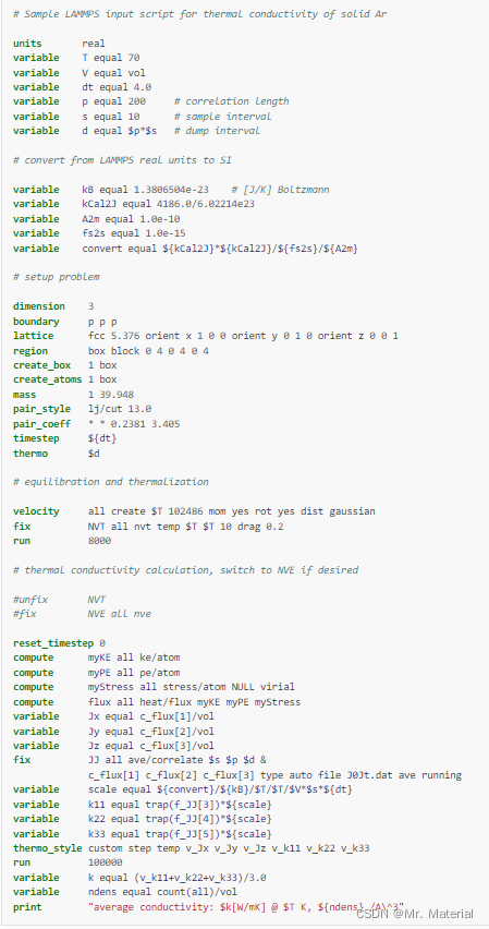
核心命令
:
\color{red}核心命令:
核心命令:
compute      myKE all ke/atom
compute      myPE all pe/atom
compute      myStress all stress/atom NULL virial
compute      flux all heat/flux myKE myPE myStress
variable     Jx equal c_flux[1]/vol
variable     Jy equal c_flux[2]/vol
variable     Jz equal c_flux[3]/vol
fix          JJ all ave/correlate $s $p $d &
             c_flux[1] c_flux[2] c_flux[3] type auto file J0Jt.dat ave running
注意:
\color{red}注意:
注意:
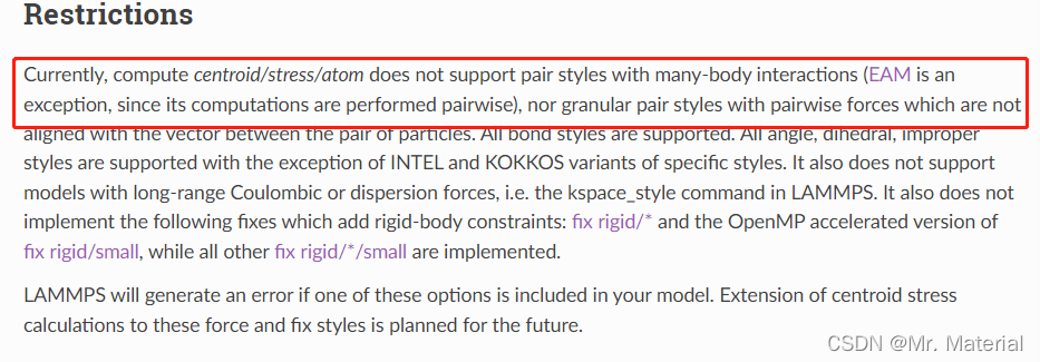
平衡态的方法主要适用于各相同性体系,计算出来的热导率是针对于无限大的体系。但是在计算位力中,
L
a
m
m
p
s
\rm Lammps
Lammps 中的命令只适用于两体势。
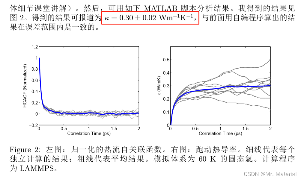
2. 报道结果
这里我们只采用结果(
60
K
A
r
的热导率
60K\ Ar的热导率
60K Ar的热导率)进行对比。
六、五种方法结果对比
感谢阅读,注意:具体问题具体分析,以下结果只提供参考!
\rm \color{red} 感谢阅读,注意:具体问题具体分析,以下结果只提供参考!
感谢阅读,注意:具体问题具体分析,以下结果只提供参考!
E
M
D
\rm EMD
EMD 计算的为
60
K
\rm 60\ K
60 K 下无限大体系的热导率;
N
E
M
D
\rm NEMD
NEMD 以及
R
N
E
M
D
\rm RNEMD
RNEMD 计算的为
10.8
n
m
\rm 10.8\ nm
10.8 nm 的热导率;


 被折叠的 条评论
为什么被折叠?
被折叠的 条评论
为什么被折叠?
 到【灌水乐园】发言


