pytorch中如何使用自己的数据集进行训练

需求

cifar10中有十个类别的图像，我需要其中的第一类和第二类作为数据集，重新构建训练集和测试集，用这份小数据集来训练一个diffusion model

get data

import os
import pickle
import numpy as np
from PIL import Image

# 替换为你的 CIFAR-10 pickle 文件路径
pickle_file_path = "train_batch_class12.pickle"

# 读取 CIFAR-10 pickle 文件内容
with open(pickle_file_path, "rb") as f:
    cifar10_data = pickle.load(f)

# 提取图像数据和标签
image_data = cifar10_data['data']
labels = cifar10_data['labels']

# 类别名称的映射字典
class_names = {
    0: "airplane",
    1: "automobile",
    # 添加其他类别的映射
}

# 循环处理每个图像
for i in range(len(image_data)):
    # 获取单个图像和对应标签
    img_array = image_data[i]
    label = labels[i]

    # 调整图像数据形状和数据类型
    img_array = img_array.reshape((3, 32, 32)).transpose((1, 2, 0))  # 调整形状和通道顺序
    img_array = img_array.astype(np.uint8)

    # 将 NumPy 数组转换为 PIL Image
    image = Image.fromarray(img_array)

    # 获取类别名称
    class_name = class_names.get(label, f"class{label}")

    # 创建存储文件夹的路径
    class_folder_path = f"train/{class_name}"
    os.makedirs(class_folder_path, exist_ok=True)

    # 保存图像到对应的类别文件夹
    image.save(os.path.join(class_folder_path, f"cifar10_image_{i}_label_{label}.png"))
    # 如果需要显示图像，取消注释下面这行
    # image.show()

import os
import pickle
import numpy as np
from PIL import Image

# 替换为你的 CIFAR-10 pickle 文件路径
pickle_file_path = "test_batch_class12.pickle"

# 读取 CIFAR-10 pickle 文件内容
with open(pickle_file_path, "rb") as f:
    cifar10_data = pickle.load(f)

# 提取图像数据和标签
image_data = cifar10_data['data']
labels = cifar10_data['labels']

# 类别名称的映射字典
class_names = {
    0: "airplane",
    1: "automobile",
    # 添加其他类别的映射
}

# 循环处理每个图像
for i in range(len(image_data)):
    # 获取单个图像和对应标签
    img_array = image_data[i]
    label = labels[i]

    # 调整图像数据形状和数据类型
    img_array = img_array.reshape((3, 32, 32)).transpose((1, 2, 0))  # 调整形状和通道顺序
    img_array = img_array.astype(np.uint8)

    # 将 NumPy 数组转换为 PIL Image
    image = Image.fromarray(img_array)

    # 获取类别名称
    class_name = class_names.get(label, f"class{label}")

    # 创建存储文件夹的路径
    class_folder_path = f"test/{class_name}"
    os.makedirs(class_folder_path, exist_ok=True)

    # 保存图像到对应的类别文件夹
    image.save(os.path.join(class_folder_path, f"cifar10_image_{i}_label_{label}.png"))
    # 如果需要显示图像，取消注释下面这行
    # image.show()

现在我们自己的数据集内的架构应该是这样的

Transforming data

在我们能够使用 PyTorch 处理图像数据之前，我们需要执行以下步骤：

1. 将图像转换为张量（图像的数值表示）tensors。
2. 将图像转换为 torch.utils.data.Dataset，然后创建一个 torch.utils.data.DataLoader。我们简称它们为 Dataset 和 DataLoader。

在深度学习中，PyTorch 的 Dataset 和 DataLoader 类是用于有效加载和处理数据的关键组件。Dataset 用于包装数据，DataLoader 则用于在训练过程中批量加载数据。这两者一起协同工作，使得数据在模型训练中更易处理。

import torch
from torch.utils.data import DataLoader
from torchvision import datasets, transforms
from pathlib import Path
from torchvision import datasets, transforms

# Write transform for image
data_transform = transforms.Compose([
    # Resize the images to 64x64
    # 我处理的是cifar10 32*32 这一步跳过
    # transforms.Resize(size=(64, 64)),
    # Flip the images randomly on the horizontal
    transforms.RandomHorizontalFlip(p=0.5), # p = probability of flip, 0.5 = 50% chance
    # Turn the image into a torch.Tensor
    transforms.ToTensor() # this also converts all pixel values from 0 to 255 to be between 0.0 and 1.0 
])



train_dir = Path("train")
test_dir = Path("test")

# Write transform for image
data_transform = transforms.Compose([
    # Resize the images to 64x64
    # 我处理的是cifar32*32 这一步跳过
    # transforms.Resize(size=(64, 64)),
    # Flip the images randomly on the horizontal
    transforms.RandomHorizontalFlip(p=0.5), # p = probability of flip, 0.5 = 50% chance
    # Turn the image into a torch.Tensor
    transforms.ToTensor() # this also converts all pixel values from 0 to 255 to be between 0.0 and 1.0 
])

train_data = datasets.ImageFolder(root=train_dir, # target folder of images
                                  transform=data_transform, # transforms to perform on data (images)
                                  target_transform=None) # transforms to perform on labels (if necessary)

test_data = datasets.ImageFolder(root=test_dir, 
                                 transform=data_transform)

print(f"Train data:\n{train_data}\nTest data:\n{test_data}")

输出为

“It looks like PyTorch has registered our Dataset’s.”

Turn loaded images into DataLoader’s

我们已经将图像转换为 PyTorch 数据集（Dataset），现在让我们使用 torch.utils.data.DataLoader 将它们转换为数据加载器。

通过将我们的数据集转换为数据加载器，我们使它们成为可迭代的，这样模型就可以遍历学习样本和目标之间的关系（特征和标签）。

import os
from torch.utils.data import DataLoader
cpu_count = os.cpu_count()
# print(f"Number of CPUs on your machine: {cpu_count}")

# Turn train and test Datasets into DataLoaders
train_dataloader = DataLoader(dataset=train_data, 
                              batch_size=32, # how many samples per batch?
                              num_workers=cpu_count, # how many subprocesses to use for data loading? (higher = more)
                              shuffle=True) # shuffle the data?

test_dataloader = DataLoader(dataset=test_data, 
                             batch_size=32, 
                             num_workers=cpu_count, 
                             shuffle=False) # don't usually need to shuffle testing data

train_dataloader, test_dataloader

img, label = next(iter(train_dataloader))

# Batch size is 32 
print(f"Image shape: {img.shape} -> [batch_size, color_channels, height, width]")
print(f"Label shape: {label.shape}")

use model tinyVGG

import torch
from torch import nn

class TinyVGG(nn.Module):
    """
    Model architecture copying TinyVGG from: 
    https://poloclub.github.io/cnn-explainer/
    """
    def __init__(self, input_shape: int, hidden_units: int, output_shape: int) -> None:
        super().__init__()
        self.conv_block_1 = nn.Sequential(
            nn.Conv2d(in_channels=input_shape, 
                      out_channels=hidden_units, 
                      kernel_size=3, # how big is the square that's going over the image?
                      stride=1, # default
                      padding=1), # options = "valid" (no padding) or "same" (output has same shape as input) or int for specific number 
            nn.ReLU(),
            nn.Conv2d(in_channels=hidden_units, 
                      out_channels=hidden_units,
                      kernel_size=3,
                      stride=1,
                      padding=1),
            nn.ReLU(),
            nn.MaxPool2d(kernel_size=2,
                         stride=2) # default stride value is same as kernel_size
        )
        self.conv_block_2 = nn.Sequential(
            nn.Conv2d(hidden_units, hidden_units, kernel_size=3, padding=1),
            nn.ReLU(),
            nn.Conv2d(hidden_units, hidden_units, kernel_size=3, padding=1),
            nn.ReLU(),
            nn.MaxPool2d(2)
        )
        self.classifier = nn.Sequential(
            nn.Flatten(),
            # Where did this in_features shape come from? 
            # It's because each layer of our network compresses and changes the shape of our inputs data.
            nn.Linear(in_features=hidden_units*8*8,
                      out_features=output_shape)
        )
    
    def forward(self, x: torch.Tensor):
        x = self.conv_block_1(x)
        # print(x.shape)
        x = self.conv_block_2(x)
        # print(x.shape)
        x = self.classifier(x)
        # print(x.shape)
        return x
        # return self.classifier(self.conv_block_2(self.conv_block_1(x))) # <- leverage the benefits of operator fusion
    
device = "cuda" if torch.cuda.is_available() else "cpu"
torch.manual_seed(42)
model_0 = TinyVGG(input_shape=3, # number of color channels (3 for RGB) 
                  hidden_units=10, 
                  output_shape=len(train_data.classes)).to(device)
model_0

原本这个模型的最后应该是如下架构

self.classifier = nn.Sequential(
    nn.Flatten(),
    nn.Linear(in_features=hidden_units * 16 * 16,
              out_features=output_shape)
)

但在 CIFAR-10 数据集中，图像的大小是 32x32，而不是硬编码的 16x16。因此，这里的 in_features 应该是 hidden_units * 8 * 8，因为通过两次最大池化后，特征图的尺寸会减半两次。

to classify

# 1. Get a batch of images and labels from the DataLoader
img_batch, label_batch = next(iter(train_dataloader))

# 2. Get a single image from the batch and unsqueeze the image so its shape fits the model
img_single, label_single = img_batch[31].unsqueeze(dim=0), label_batch[31]
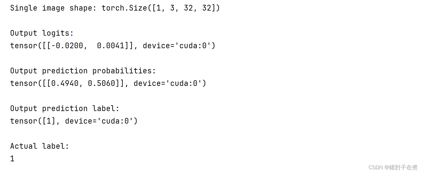
print(f"Single image shape: {img_single.shape}\n")

# 3. Perform a forward pass on a single image
model_0.eval()
with torch.inference_mode():
    pred = model_0(img_single.to(device))
    
# 4. Print out what's happening and convert model logits -> pred probs -> pred label
print(f"Output logits:\n{pred}\n")
print(f"Output prediction probabilities:\n{torch.softmax(pred, dim=1)}\n")
print(f"Output prediction label:\n{torch.argmax(torch.softmax(pred, dim=1), dim=1)}\n")
print(f"Actual label:\n{label_single}")

问题

这里数据集已经可以进入模型了，但是并没有训练这个模型。