


前言
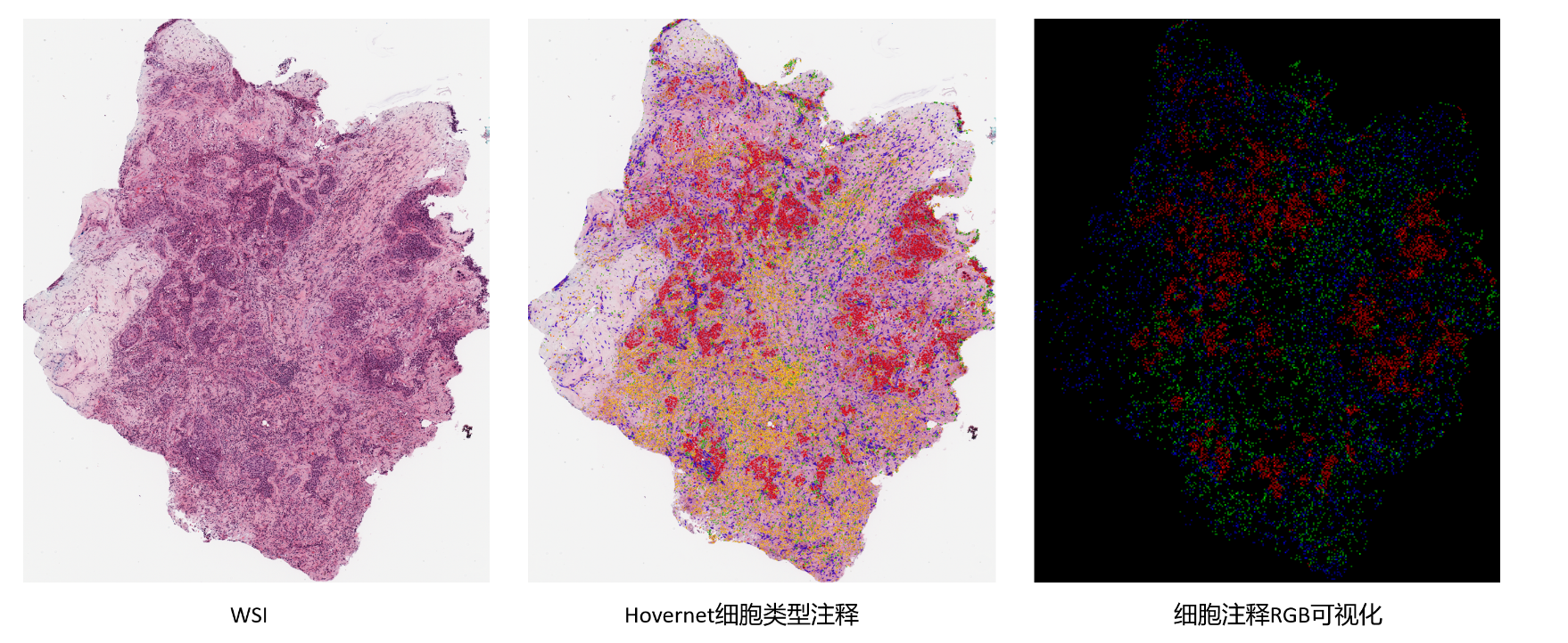
Hovernet按svs格式的WSI分别识别图像类型,速度慢。因此,尝试将整图WSI转为png进行细胞识别(纯属个人试试)并进行RGB可视化。
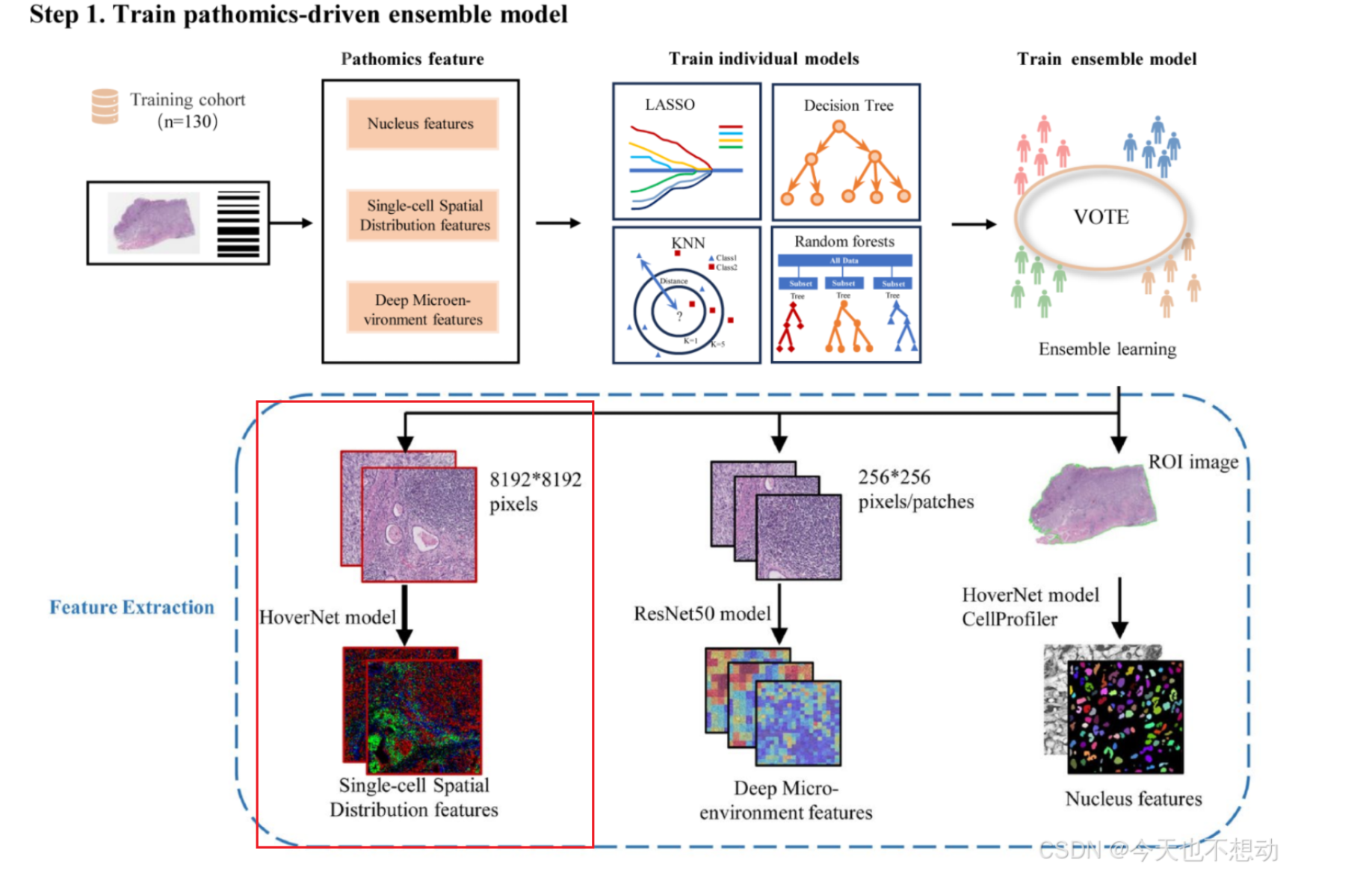
RGB可视化这步属于Development and interpretation of a pathomics-driven ensemble model for predicting the response to immunotherapy in gastric cancer中三种特征提取方式之一的部分实操复现(如下图红框位置)。
** 具体代码实现 **
Step1: 统计病理切片属性信息
import openslide
import matplotlib.pyplot as plt
import os
import numpy as np
import pandas as pd

data_dir ="../input_dataset/"

dir_lst = os.listdir(data_dir)
dir_lst = [i for i in dir_lst if i.endswith("ndpi")]
print(len(dir_lst))

df_wsi = pd.DataFrame(columns = ["Slide name","Level_0_magnification", "Dimensions","Level count", "Level dimensions","Level downsamples"])
for file in dir_lst:
    svs_file_path = data_dir + file
    slide = openslide.OpenSlide(svs_file_path)
    downsample_lst = [int(i) for i in list(slide.level_downsamples)]
    app_mag = slide.properties.get('aperio.AppMag', 40)  # 如果不存在,返回 'Unknown'
#     print(app_mag,svs_file_path)
    info = [file,int(app_mag),slide.dimensions,slide.level_count,slide.level_dimensions ,downsample_lst ]

    df_wsi.loc[len(df_wsi)] = info
# df_wsi.to_csv("slide_stat.csv",index=False)
df_wsi.head()
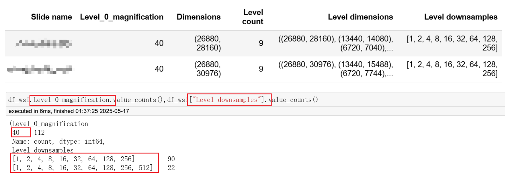
结果表示所有图像最大分辨率为40X,下采样级别为[1,2,4,8…]。代表可以获得放大倍数为40X,20X,10X等的图像。
这步的目的是明确图像的属性,不同批次的病理切片属性不一样,分析时需要注意。
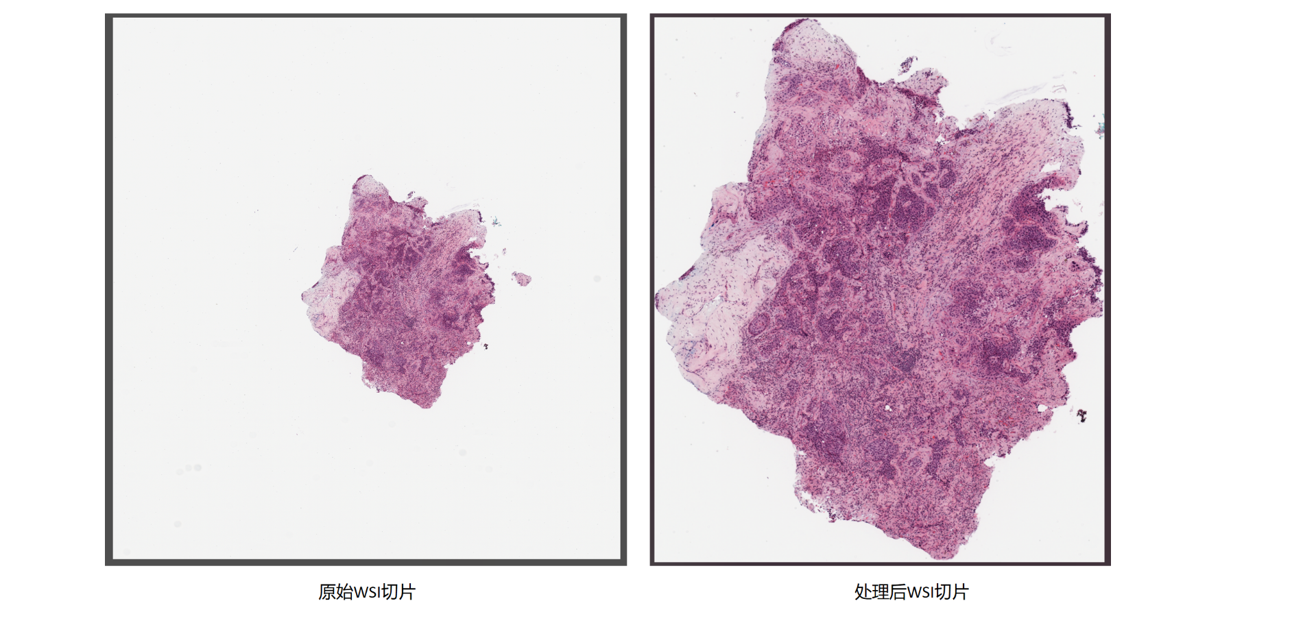
Step2: WSI转png,(尽量)去除非组织部分(减少文件大小)
转svs为png
import openslide
import numpy as np
from PIL import Image
import os

def convert_svs_to_png(svs_path, output_folder):
    slide = openslide.open_slide(svs_path)

    # 获取最大分辨率下的图像尺寸
#     width, height = slide.dimensions
    patch_level = 2 # 这里是20x
    width, height = list(df_wsi[df_wsi["Slide name"]==os.path.basename(svs_path)]["Level dimensions"])[0][patch_level]
    img = slide.read_region((0, 0), patch_level, (width, height)) # 坐标 层级(层级 0 是最高分辨率)读取的图像区域的宽度和高度
    img = slide.read_region((0, 0), patch_level, (width, height))

    img_array = np.array(img)

    # 保存为 PNG 格式
    output_path = os.path.join(output_folder, os.path.basename(svs_path).replace('.ndpi', '.png'))
    Image.fromarray(img_array).save(output_path)

output_dir = './png_Level_0_magnification'
if not os.path.exists(output_dir):
    os.makedirs(output_dir)
for svs_file in os.listdir(data_dir):
    if not os.path.isfile(os.path.join(output_dir,svs_file.replace('.ndpi', '.png'))):
        svs_file = data_dir + svs_file
        print(svs_file)
        convert_svs_to_png(svs_file, output_dir)
保留组织块,且像素长宽能被16整除
import cv2
import numpy as np

def remove_whitespace_from_image(image_path, output_path):
    # 读取图像
    image = cv2.imread(image_path)
    if image is None:
        print("无法读取图像,请检查路径是否正确。")
        return

    # 转换为灰度图像
    gray = cv2.cvtColor(image, cv2.COLOR_BGR2GRAY)

    # 使用阈值分割去除偏白色区域(可根据实际调整阈值)
    _, thresh = cv2.threshold(gray, 240, 255, cv2.THRESH_BINARY)

    # 反转图像,将白色背景变为黑色,组织区域变为白色
    thresh = cv2.bitwise_not(thresh)

    # 寻找轮廓
    contours, _ = cv2.findContours(thresh, cv2.RETR_EXTERNAL, cv2.CHAIN_APPROX_SIMPLE)

    # 获取最大轮廓(假设组织区域是最大的连通区域)
    if contours:
        max_contour = max(contours, key=cv2.contourArea)
        x, y, w, h = cv2.boundingRect(max_contour)

        # 裁剪图像
        cropped_image = image[y:y+h, x:x+w]

        # 保证裁剪后的图像尺寸能被 16 整除
        height, width = cropped_image.shape[:2]

        # 计算需要裁剪的像素数量
        width_remainder = width % 16
        height_remainder = height % 16

        # 如果宽度不能被 16 整除,则从左右两侧均匀裁剪
        if width_remainder != 0:
            width_crop_left = width_remainder // 2
            width_crop_right = width_remainder - width_crop_left
            cropped_image = cropped_image[:, width_crop_left:width - width_crop_right]

        # 如果高度不能被 16 整除,则从上下两侧均匀裁剪
        if height_remainder != 0:
            height_crop_top = height_remainder // 2
            height_crop_bottom = height_remainder - height_crop_top
            cropped_image = cropped_image[height_crop_top:height - height_crop_bottom, :]

        cv2.imwrite(output_path, cropped_image)
        print(f"处理完成,裁剪后的图像已保存到 {output_path}, 像素大小为 {cropped_image.shape}, 宽能被16整除吗: {cropped_image.shape[1] % 16 == 0}, 高能被16整除吗: {cropped_image.shape[0] % 16 == 0}")

    else:
        print("未找到组织区域,请检查图像或调整阈值。")

# 示例运行
from tqdm import tqdm
for png_file in tqdm(os.listdir(output_dir)):
    if png_file.endswith('.png') and '_tissue' not in png_file and not os.path.exists(os.path.join(output_dir,png_file.replace('.png','_tissue.png'))):
        input_image_path = os.path.join(output_dir, png_file)
        output_image_path  = os.path.join(output_dir, png_file.replace('.png','_tissue.png'))
        print(input_image_path)
        print(output_image_path)
        remove_whitespace_from_image(input_image_path, output_image_path)
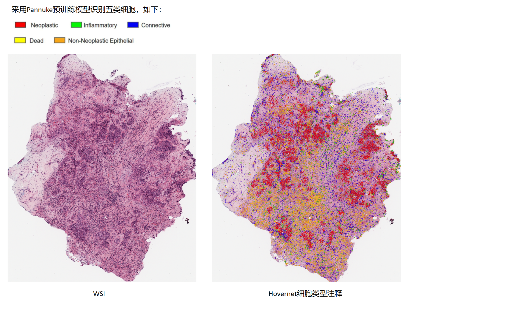
Step3:采用hovernet tile模型进行细胞类型识别
## input_dataset_tiles为放置输入图片(png)的文件夹。执行细胞分割识别任务时,自动生成输出文件output_tiles_Pannuke ##

# 在run_infer.py文件中加入下续命令
import torch.multiprocessing
torch.multiprocessing.set_sharing_strategy('file_system')

# 执行细胞分割任务
python run_infer.py --gpu='0' --nr_types=6 --type_info_path='type_info_pannuke.json'  --model_path='./hover-net-pytorch-weights/hovernet_fast_pannuke_type_tf2pytorch.tar' --model_mode='fast' --nr_inference_workers=8 --nr_post_proc_workers=16 --batch_size=1  tile --input_dir='./input_dataset_tiles/' --output_dir='./output_tiles_Pannuke/' --mem_usage=0.1 --draw_dot --save_qupath

# 若报错一次可执行下述命令再运行
ls output_tiles_Pannuke/overlay/ | while read i;do rm input_dataset_tiles/$i; done
python run_infer.py --gpu='0' --nr_types=6 --type_info_path='type_info_pannuke.json'  --model_path='./hover-net-pytorch-weights/hovernet_fast_pannuke_type_tf2pytorch.tar' --model_mode='fast' --nr_inference_workers=8 --nr_post_proc_workers=16 --batch_size=1  tile --input_dir='./input_dataset_tiles/' --output_dir='./output_tiles_Pannuke_tmp/' --mem_usage=0.1 --draw_dot --save_qupath

# 若再再报错,先执行下续命令,再依次执行上述两行命令
rsync -av --include '*/' --include '*.*' --exclude '*' ./output_tiles_Pannuke_tmp/ ./output_tiles_Pannuke/ # 递归的将./output_tiles_Pannuke_tmp/目录的文件转移到./output_tiles_Pannuke/中
Step4:RGB可视化
实现思路:在图片按64*64的方格进行滑窗,计算每个滑窗内不同类型细胞的数量。RGB图三层三种颜色分别代表一种细胞类型,颜色可区分细胞类型,亮度可区分细胞密度。
单张图片示例如下:
# load the libraries

import sys
sys.path.append('../hover_net/')

import numpy as np
import pandas as pd
import os
import glob
import matplotlib.pyplot as plt
import scipy.io as sio
import cv2
import json
import openslide
import shutil
import os
from misc.wsi_handler import get_file_handler
from misc.viz_utils import visualize_instances_dict


tile_path = './hover_net/input_dataset_tiles///'
tile_json_path = './hover_net/output_tiles_Pannuke//json/'
tile_mat_path = './hover_net/output_tiles_Pannuke//mat/'
tile_overlay_path  = './hover_net/output_tiles_Pannuke//overlay/'


Single_cell_spatial_distribution_map_dir = "./Single_cell_spatial_distribution_map/"
if os.path.exists(Single_cell_spatial_distribution_map_dir):
    shutil.rmtree(Single_cell_spatial_distribution_map_dir)
os.makedirs(Single_cell_spatial_distribution_map_dir)


from PIL import Image

image_path = tile_overlay_path +"C3L-01663-21_tissue.png"
image = Image.open(image_path)

width, height = image.size
print(width, height)
# 获取图片的DPI(如果存在)
dpi = info.get("dpi", (64, 64))  # 默认值为64/32 DPI
print(dpi)
import numpy as np
import cv2
import json  # 用于加载 JSON 格式的 HoverNet 输出

def create_rgb_density_map_from_hovernet(hovernet_output, image_size=(256, 256), grid_size=(16, 16)):
    """
    基于 HoverNet 输出创建 RGB 密度图。

    Args:
        hovernet_output (dict): HoverNet 的输出,包含细胞位置和类型信息。
        image_size (tuple): 图像的尺寸 (width, height)。
        grid_size (tuple): 网格的尺寸 (width, height)。

    Returns:
        numpy.ndarray:RGB 图像 (NumPy 数组)。
    """

    # 1. 细胞类型映射
    cell_type_map = {
        1: "tumor",  # 假设 1 代表肿瘤细胞
        3: "stromal",  # 假设 2 代表基质细胞
        2: "lymphocyte",  # 假设 4 代表淋巴细胞
        # 可以根据实际 HoverNet 输出添加更多类型
    }

    # 2. 创建网格
    num_grid_rows = image_size[1] // grid_size[1]  # 256 // 64 = 4
    num_grid_cols = image_size[0] // grid_size[0]  # 256 // 64 = 4

    # 3. 初始化网格计数器
    grid_counts = np.zeros((num_grid_rows, num_grid_cols, 3), dtype=np.int32)  # [R,G,B]

    # 4. 统计细胞数量
    for cell_id, cell_info in hovernet_output['nuc'].items(): # 遍历每个细胞
        cell_type_id = cell_info['type']
        if cell_type_id in cell_type_map: #只统计我们关心的细胞类型
            cell_type = cell_type_map[cell_type_id]
            centroid = cell_info['centroid']  # 获取细胞质心坐标 (x, y)
            x, y = int(centroid[0]), int(centroid[1])

            if 0 <= x < image_size[0] and 0 <= y < image_size[1]:
                grid_col = x // grid_size[0]
                grid_row = y // grid_size[1]

                if 0 <= grid_row < num_grid_rows and 0 <= grid_col < num_grid_cols:
                    if cell_type == "tumor":
                        grid_counts[grid_row, grid_col, 0] += 1
                    elif cell_type == "lymphocyte":
                        grid_counts[grid_row, grid_col, 1] += 1
                    elif cell_type == "stromal":
                        grid_counts[grid_row, grid_col, 2] += 1

    # 5. 创建 RGB 图像
    rgb_image = np.zeros((num_grid_rows, num_grid_cols, 3), dtype=np.uint8)

    # 遍历每个网格
    for i in range(num_grid_rows):
        for j in range(num_grid_cols):
            # 获取当前网格的细胞数量
            tumor_count = grid_counts[i, j, 0]
            lymphocyte_count = grid_counts[i, j, 1]
            stromal_count = grid_counts[i, j, 2]

            # 映射细胞数量到 RGB 值 (0-255)
            # 这里可以根据需求调整映射方式
            max_count = 2  # 设置一个最大细胞数量阈值,超过这个阈值的都设为 255
            red = min(int(tumor_count * (255 / max_count)), 255)
            green = min(int(lymphocyte_count * (255 / max_count)), 255)
            blue = min(int(stromal_count * (255 / max_count)), 255)

            rgb_image[i, j] = [blue, green, red]  # 注意 OpenCV 的颜色通道顺序是 BGR

    # 将图像放大到原始尺寸,方便可视化
    rgb_image = cv2.resize(rgb_image, image_size, interpolation=cv2.INTER_NEAREST)  # 使用最近邻插值
    print("Image size:", image_size)
    print("Grid size:", grid_size)
    print("Number of grid rows and cols:", num_grid_rows, num_grid_cols)
    return rgb_image
# 示例用法:
if __name__ == '__main__':
    # 1. 加载 HoverNet 输出 (假设保存在 JSON 文件中)
    hovernet_output_file = "./hover_net/output_tiles_Pannuke//json/C3L-01663-21_tissue.json"  # 替换为你的文件名
    with open(hovernet_output_file, 'r') as f:
        hovernet_output = json.load(f)

    # 使用你提供的 HoverNet 输出作为示例
    image_path = tile_overlay_path + "C3L-01663-21_tissue.png"
    image = Image.open(image_path)

    image_size = image.size
    print(image_size)
    grid_size = (16, 16)

    # 2. 创建 RGB 密度图
    rgb_image = create_rgb_density_map_from_hovernet(hovernet_output, image_size, grid_size)

    # 3. 保存图像
    outfile = Single_cell_spatial_distribution_map_dir + os.path.basename(hovernet_output_file).replace(".json",".png")
    cv2.imwrite(outfile, rgb_image)
    print("RGB density map saved as ", outfile)
Step5:深度学习预训练模型提取图片特征
细胞注释RGB可视化后,可参考文献 “Development and interpretation of a pathomics-driven ensemble model for predicting the response to immunotherapy in gastric cancer” 采用深度学习方法进行特征 (Single-cell_spatial_distribution_pathomics_features) 提取。


 被折叠的 条评论
为什么被折叠?
被折叠的 条评论
为什么被折叠?
 到【灌水乐园】发言


