多目标跟踪BOT-SORT算法（卡尔曼滤波）

卡尔曼滤波（Kalman Filter）是一种递归滤波算法，常用于在噪声和不确定性中估计系统的状态。它是基于状态空间模型，利用观测数据和系统的动态模型来估计系统的状态。卡尔曼滤波通常用于导航、控制、时间序列预测等领域。

1. 卡尔曼滤波的基本概念

卡尔曼滤波是一种最优估计方法，能够通过已知的系统模型和测量值来估计未知的状态，并且不断地更新估计值。其核心思想是利用当前的测量值和先前的估计值结合，得出一个最优的估计结果。

2. 卡尔曼滤波的基本模型

假设有一个动态系统，系统的状态可以通过以下方程进行描述：

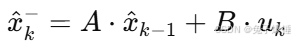
2.1 状态方程

• 表示在时间 kkk 时刻的系统状态。
• A 是状态转移矩阵，表示从时间 k−1k-1k−1 到时间 kkk 的系统状态转移关系。
• B 是控制输入矩阵，表示控制输入对状态的影响。
•  是控制输入。
•  是过程噪声，通常假设是零均值、高斯分布的白噪声。

2.2 观测方程

•  是在时间 kkk 时刻的观测值。
• H 是观测矩阵，描述了如何从状态 xkx_kxk​ 得到观测值 zkz_kzk​。
• 是观测噪声，通常也是零均值、高斯分布的白噪声。

3. 卡尔曼滤波的递归过程

卡尔曼滤波通过两个步骤来更新状态估计：预测步骤和更新步骤。

3.1 预测步骤

在预测步骤中，根据当前的状态估计和控制输入来预测系统的下一个状态。

• 预测当前状态：

  

• 预测当前误差协方差：

  

   

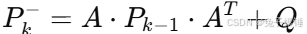
  其中， 是误差协方差矩阵，描述了状态估计的不确定性，Q 是过程噪声协方差矩阵。

3.2 更新步骤

在更新步骤中，根据观测数据对预测的状态进行修正。

• 计算卡尔曼增益：

  

  其中，R 是观测噪声协方差矩阵。

• 更新估计值：

  

• 更新误差协方差矩阵：

  

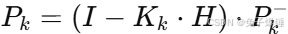
  其中，I 是单位矩阵。

4. 卡尔曼滤波的优势

• 最优性：卡尔曼滤波在满足系统噪声满足高斯分布、系统模型准确的情况下，能够提供最优的状态估计。
• 递归性：卡尔曼滤波是一种递归算法，只依赖于最新的测量数据和上一步的估计结果，不需要存储所有历史数据。
• 实时性：卡尔曼滤波适用于实时估计，可以迅速更新状态估计。

5. 卡尔曼滤波的应用

卡尔曼滤波在多个领域有广泛应用，主要包括：

• 导航与定位：例如GPS和IMU传感器的数据融合，卡尔曼滤波常用于估计飞机、无人机、机器人等的当前位置和姿态。
• 金融领域：用来进行股市预测、时间序列分析等。
• 控制系统：用于控制系统中的状态估计，例如机器人的运动控制。
• 信号处理：例如去噪声、滤波等。

6. 扩展卡尔曼滤波（EKF）与无迹卡尔曼滤波（UKF）

卡尔曼滤波的基本模型假设系统是线性的，但在实际应用中，许多系统是非线性的。为此，发展出了扩展卡尔曼滤波（EKF）和无迹卡尔曼滤波（UKF）。

• 扩展卡尔曼滤波（EKF）：对非线性系统进行一阶泰勒展开近似，线性化处理非线性部分。
• 无迹卡尔曼滤波（UKF）：通过确定一组采样点来近似非线性系统的分布，避免了线性化过程。

这些方法可以用于更复杂的、非线性的系统状态估计问题。

7. 卡尔曼滤波在多目标跟踪算法中的作用

根据上一帧的对象检测结果，推断下一帧对象所在的位置。

8. 卡尔曼滤波在BOT-SORT算法中的代码及注释

# vim: expandtab:ts=4:sw=4
import numpy as np
import scipy.linalg


"""
Table for the 0.95 quantile of the chi-square distribution with N degrees of freedom (contains values for N=1, ..., 9).
Taken from MATLAB/Octave's chi2inv function and used as Mahalanobis gating threshold.
N个自由度的卡方分布的0.95分位数的表(包含N=1，…， 9).取自MATLAB/Octave的chi2inv函数，作为并用作马氏(Mahalanobis)选通阈值
"""
chi2inv95 = {
    1: 3.8415,
    2: 5.9915,
    3: 7.8147,
    4: 9.4877,
    5: 11.070,
    6: 12.592,
    7: 14.067,
    8: 15.507,
    9: 16.919}


class KalmanFilter(object):
    """
    A simple Kalman filter for tracking bounding boxes in image space.
    一个简单的卡尔曼滤波器用于跟踪图像空间中的包围框。
    The 8-dimensional state space
        x, y, w, h, vx, vy, vw, vh
    contains the bounding box center position (x, y), width w, height h, and their respective velocities.
    8维状态空间包含边界框中心位置(x, y)、宽度w、高度h以及它们各自的速度。

    Object motion follows a constant velocity model. The bounding box location (x, y, w, h) is taken as direct observation of the state space (linear observation model).
    物体运动遵循匀速模型。取边界盒位置(x, y, w, h)作为状态空间的直接观测(线性观测模型)。

    卡尔曼滤波器在Deep SORT中，需要估计Track的以下状态：
        •均值：用8维向量（x, y, a, h, vx, vy, va, vh）表示。(x,y)是框的中心坐标，宽高比是a,高度h以及对应的速度，所有的速度都将初始化为0。
        •协方差：表示目标位置信息的不确定程度，用8x8的对角矩阵来表示，矩阵对应的值越大，代表不确定程度越高
    """

    def __init__(self):
        """
        self._motion_mat    A矩阵   卡尔曼中的运动转移矩阵，也就是状态转移矩阵
        self._update_mat    H矩阵   卡尔曼中的 观测矩阵
        self._std_weight_position，self._std_weight_velocity是Q、R调整参数
        """
        ndim, dt = 4, 1.

        # Create Kalman filter model matrices.
        # 创建状态转移矩阵 A 或者 F
        self._motion_mat = np.eye(2 * ndim, 2 * ndim)
        for i in range(ndim):
            self._motion_mat[i, ndim + i] = dt
            # 其中self._motion_mat中存的为卡尔曼中的A矩阵，其具体值为上文现实的样子（为什么是这样，是因为建模就是这样建立的，建立了一个恒定速度的模型）
            # _motion_mat = [[1, 0, 0, 0, dt, 0, 0, 0],
            #                [0, 1, 0, 0, 0, dt, 0, 0],
            #                [0, 0, 1, 0, 0, 0, dt, 0],
            #                [0, 0, 0, 1, 0, 0, 0, dt],
            #                [0, 0, 0, 0, 1, 0, 0, 0],
            #                [0, 0, 0, 0, 0, 1, 0, 0],
            #                [0, 0, 0, 0, 0, 0, 1, 0],
            #                [0, 0, 0, 0, 0, 0, 0, 1],
            #                ]   A矩阵   卡尔曼中的运动转移矩阵，也就是状态转移矩阵
        self._update_mat = np.eye(ndim, 2 * ndim)
        # 其中self._update_mat是卡尔曼中的观测矩阵，这个很好理解 Z=HX（这是矩阵乘法，不可以随意调换顺序）
        # _update_mat = [[1, 0, 0, 0, 0, 0, 0, 0],
        #                [0, 1, 0, 0, 0, 0, 0, 0],
        #                [0, 0, 1, 0, 0, 0, 0, 0],
        #                [0, 0, 0, 1, 0, 0, 0, 0],
        #                ]    H 矩阵   卡尔曼中的 观测矩阵

        # Motion and observation uncertainty are chosen relative to the current state estimate.
        # These weights control the amount of uncertainty in the model. This is a bit hacky.
        # 其中，self._std_weight_position，self._std_weight_velocity是Q、R调整参数
        self._std_weight_position = 1. / 20  # Q、R调整参数，仅仅是调整参数
        self._std_weight_velocity = 1. / 160

    def initiate(self, measurement):  # xywh
        """Create track from unassociated measurement. 从无关联测量创建轨迹
        Parameters
        ----------
        measurement : ndarray
            Bounding box coordinates (x, y, w, h) with center position (x, y), width w, and height h.
        Returns
        -------
        (ndarray, ndarray)
            Returns the mean vector (8 dimensional) and covariance matrix (8x8 dimensional) of the new track. Unobserved velocities are initialized to 0 mean.
            返回新轨迹的平均向量（8维）和协方差矩阵（8x8维）。未观测到的速度初始化为平均值0。
        mean    X 状态向量
        covariance  P矩阵   只要不是0矩阵就可以  P也就是协方差矩阵
        """
        mean_pos = measurement  # [714.96710205 792.23687744 101.25 220.26318359] 中点，xy与宽高wh
        mean_vel = np.zeros_like(mean_pos)  # mean_vel: [0. 0. 0. 0.]
        mean = np.r_[mean_pos, mean_vel]  # 初始化状态向量 mean，mean: [714.96710205 792.23687744 101.25 220.26318359 0. 0. 0. 0.]

        std = [  # 此处 与 StrongSORT 不一样。 std: [10.125, 22.026318359375, 10.125, 22.026318359375, 6.328125, 13.766448974609375, 6.328125, 13.766448974609375]
            2 * self._std_weight_position * measurement[2],
            2 * self._std_weight_position * measurement[3],
            2 * self._std_weight_position * measurement[2],
            2 * self._std_weight_position * measurement[3],
            10 * self._std_weight_velocity * measurement[2],
            10 * self._std_weight_velocity * measurement[3],
            10 * self._std_weight_velocity * measurement[2],
            10 * self._std_weight_velocity * measurement[3]]
        covariance = np.diag(np.square(std))  # 对std平方后，化为对角矩阵
        return mean, covariance
        # covariance = [[(2 * self._std_weight_position * measurement[2]) ** 2, 0, 0, 0, 0, 0, 0, 0],
        #               [0, (2 * self._std_weight_position * measurement[3]) ** 2, 0, 0, 0, 0, 0, 0],
        #               [0, 0, (2 * self._std_weight_position * measurement[2]) ** 2, 0, 0, 0, 0, 0],
        #               [0, 0, 0, (2 * self._std_weight_position * measurement[3]) ** 2, 0, 0, 0, 0],
        #               [0, 0, 0, 0, (10 * self._std_weight_velocity * measurement[2]) ** 2, 0, 0, 0],
        #               [0, 0, 0, 0, 0, (10 * self._std_weight_velocity * measurement[3]) ** 2, 0, 0],
        #               [0, 0, 0, 0, 0, 0, (10 * self._std_weight_velocity * measurement[2]) ** 2, 0],
        #               [0, 0, 0, 0, 0, 0, 0, (10 * self._std_weight_velocity * measurement[3]) ** 2],
        #               ]   初始化P矩阵   只要不是0矩阵就可以  P也就是协方差矩阵

    def predict(self, mean, covariance):
        """Run Kalman filter prediction step.  运行卡尔曼滤波预测步骤。
        Parameters
        ----------
        mean : ndarray
            The 8 dimensional mean vector of the object state at the previous time step.
            在前一个时间步的对象状态的8维平均向量。
        covariance : ndarray
            The 8x8 dimensional covariance matrix of the object state at the previous time step.
            前一个时间步的对象状态的8x8维协方差矩阵。
        Returns
        -------
        (ndarray, ndarray)
            Returns the mean vector and covariance matrix of the predicted state. Unobserved velocities are initialized to 0 mean.
            返回预测状态的平均向量和协方差矩阵。未观测速度初始化为0均值。
        """
        std_pos = [  # 不一样！！！！！！！！！！！
            self._std_weight_position * mean[2],
            self._std_weight_position * mean[3],
            self._std_weight_position * mean[2],
            self._std_weight_position * mean[3]]
        std_vel = [  # 不一样！！！！！！！！！！！
            self._std_weight_velocity * mean[2],
            self._std_weight_velocity * mean[3],
            self._std_weight_velocity * mean[2],
            self._std_weight_velocity * mean[3]]
        motion_cov = np.diag(np.square(np.r_[std_pos, std_vel]))

        mean = np.dot(mean, self._motion_mat.T)  # 不一样！！！！！！！！！！！
        covariance = np.linalg.multi_dot((
            self._motion_mat, covariance, self._motion_mat.T)) + motion_cov

        return mean, covariance

    def project(self, mean, covariance):  # mean:[714.79743843 792.75223845 101.30253632 220.20915162 0. 0. 0. 0.]  covariance:是8*8矩阵
        """Project state distribution to measurement space.  将状态分布投影到测量空间。
        Parameters
        ----------
        mean : ndarray
            The state's mean vector (8 dimensional array).
        covariance : ndarray
            The state's covariance matrix (8x8 dimensional).
        Returns
        -------
        (ndarray, ndarray)
            Returns the projected mean and covariance matrix of the given state estimate.
            返回给定状态的投影平均值和协方差矩阵
        """
        # R测量过程中噪声的协方差
        std = [  # 不一样！！！！！！！！！！！
            self._std_weight_position * mean[2],
            self._std_weight_position * mean[3],
            self._std_weight_position * mean[2],
            self._std_weight_position * mean[3]]  # list:4

        # 初始化噪声矩阵 R
        innovation_cov = np.diag(np.square(std))  # 其中 innovation_cov为 R  测量噪声协方差 4*4

        # 将均值向量映射到检测空间，即 Hx'
        mean = np.dot(self._update_mat, mean)  # mean = H(4*8) X(8,)  结果mean：4
        # 将协方差矩阵映射到检测空间，即 HP'H^T
        covariance = np.linalg.multi_dot((
            self._update_mat, covariance, self._update_mat.T))  # 噪声协方差矩阵的传递  covariance结果4*4
        return mean, covariance + innovation_cov  # 返回给定状态的投影平均值和协方差矩阵

    def multi_predict(self, mean, covariance):  # StrongSORT 中都没有这个函数    不一样！！！！！！！！！！！
        """Run Kalman filter prediction step (Vectorized version).  运行卡尔曼滤波预测步骤(矢量化版本)。
        Parameters
        ----------
        mean : ndarray
            The Nx8 dimensional mean matrix of the object states at the previous time step.
            在前一个时间步中对象状态的Nx8维平均矩阵。
        covariance : ndarray
            The Nx8x8 dimensional covariance matrics of the object states at the previous time step.
            在前一个时间步骤中对象状态的Nx8x8维协方差矩阵。
        Returns
        -------
        (ndarray, ndarray)
            Returns the mean vector and covariance matrix of the predicted state. Unobserved velocities are initialized to 0 mean.
            返回预测状态的平均向量和协方差矩阵。未观测速度初始化为0均值。
        """
        std_pos = [
            self._std_weight_position * mean[:, 2],
            self._std_weight_position * mean[:, 3],
            self._std_weight_position * mean[:, 2],
            self._std_weight_position * mean[:, 3]]
        std_vel = [
            self._std_weight_velocity * mean[:, 2],
            self._std_weight_velocity * mean[:, 3],
            self._std_weight_velocity * mean[:, 2],
            self._std_weight_velocity * mean[:, 3]]
        sqr = np.square(np.r_[std_pos, std_vel]).T  # np.r_是按列连接两个矩阵，就是把两矩阵上下相加，要求列数相等。 np.c_是按行连接两个矩阵，就是把两矩阵左右相加，要求行数相等

        motion_cov = []
        for i in range(len(mean)):
            motion_cov.append(np.diag(sqr[i]))
        motion_cov = np.asarray(motion_cov)  # 主要区别在于 np.array（默认情况下）将会copy该对象，而 np.asarray除非必要，否则不会copy该对象
        # motion_cov 是 预测噪声协方差矩阵
        mean = np.dot(mean, self._motion_mat.T)  # X = A * X    x' = Fx ?????????????????????????????
        left = np.dot(self._motion_mat, covariance).transpose((1, 0, 2))  # AP
        covariance = np.dot(left, self._motion_mat.T) + motion_cov  # P = FPF + Q       P' = FPF^T+Q

        return mean, covariance  # 返回预测 期望中值、协方差矩阵

    def update(self, mean, covariance, measurement):
        """Run Kalman filter correction step. 运行卡尔曼滤波器校正步骤。
        Parameters
        ----------
        mean : ndarray
            The predicted state's mean vector (8 dimensional). 预测状态的平均向量（8维）
        covariance : ndarray
            The state's covariance matrix (8x8 dimensional). 状态的协方差矩阵（8x8维）
        measurement : ndarray
            The 4 dimensional measurement vector (x, y, w, h), where (x, y) is the center position, w the width, and h the height of the bounding box.
            4维测量向量(x, y, w, h)，其中(x, y)是中心位置，w是宽度，h是包围框的高度。
        Returns
        -------
        (ndarray, ndarray)
            Returns the measurement-corrected state distribution. 返回测量校正的状态分布
        """
        # mean, covariance是预测的
        # projected_mean shape：4, projected_cov shape：4*4，预测值转换到测量空间
        projected_mean, projected_cov = self.project(mean, covariance)  # 返回给定状态的投影平均值和协方差矩阵 不一样！！！！！！！！！！！

        # 该部分为卡尔曼增益求解
        # K(HPH'+R)=PH'   其中 (HPH'+R) 的值就是projected_cov （定义为S的话）
        chol_factor, lower = scipy.linalg.cho_factor(
            projected_cov, lower=True, check_finite=False)  # 返回包含 Hermitian 正定矩阵 a 的 Cholesky 分解 A = L L* 或 A = U* U 的矩阵
        kalman_gain = scipy.linalg.cho_solve(
            (chol_factor, lower), np.dot(covariance, self._update_mat.T).T,
            check_finite=False).T
        innovation = measurement - projected_mean  # Z - HX

        new_mean = mean + np.dot(innovation, kalman_gain.T)  # X + K(Z - HX)
        new_covariance = covariance - np.linalg.multi_dot((
            kalman_gain, projected_cov, kalman_gain.T))  # 预测P - KH PKT
        return new_mean, new_covariance

    def gating_distance(self, mean, covariance, measurements,
                        only_position=False, metric='maha'):    # 这个函数参数和结构都不一样！！！！！！！！！！！
        """Compute gating distance between state distribution and measurements.
        A suitable distance threshold can be obtained from `chi2inv95`. If `only_position` is False, the chi-square distribution has 4 degrees of freedom, otherwise 2.
        从' chi2inv95 '可以得到一个合适的距离阈值。如果' only_position '为False，则卡方分布的自由度为4，否则为2。
        Parameters
        ----------
        mean : ndarray
            Mean vector over the state distribution (8 dimensional).
        covariance : ndarray
            Covariance of the state distribution (8x8 dimensional).
        measurements : ndarray
            An Nx4 dimensional matrix of N measurements, each in
            format (x, y, a, h) where (x, y) is the bounding box center
            position, a the aspect ratio, and h the height.
        only_position : Optional[bool]
            If True, distance computation is done with respect to the bounding
            box center position only.
        Returns
        -------
        ndarray
            Returns an array of length N, where the i-th element contains the
            squared Mahalanobis distance between (mean, covariance) and
            `measurements[i]`.
        """
        mean, covariance = self.project(mean, covariance)
        if only_position:
            mean, covariance = mean[:2], covariance[:2, :2]
            measurements = measurements[:, :2]

        d = measurements - mean
        if metric == 'gaussian':
            return np.sum(d * d, axis=1)
        elif metric == 'maha':
            cholesky_factor = np.linalg.cholesky(covariance)
            z = scipy.linalg.solve_triangular(
                cholesky_factor, d.T, lower=True, check_finite=False,
                overwrite_b=True)
            squared_maha = np.sum(z * z, axis=0)
            return squared_maha
        else:
            raise ValueError('invalid distance metric')

 总结

卡尔曼滤波是一种强大而高效的递归滤波器，适用于估计动态系统的状态，尤其是在存在噪声和不确定性的情况下。它的优势在于能够提供最优估计，并且能够在实时系统中有效运行。

参考链接：

https://mp.weixin.qq.com/s?__biz=MzU1NjEwMTY0Mw==&mid=2247569980&idx=1&sn=1dc0b

392d32930733243c1b5a98e17d1&chksm=fbc9ab58ccbe224ea9039030453970362bd9306c7f43eccffc80d638a9bff826e94c0bc0be64&scene=27

https://blog.csdn.net/u010712012/article/details/90294295

NirAharon/BoT-SORT: BoT-SORT: Robust Associations Multi-Pedestrian Tracking