


1 用到的包
导入在这个分配过程中需要的所有包。
- Numpy 是使用 Python 进行科学计算的基本软件包。
- Matplotlib 是在 Python 中绘制图形的流行库。
- tensorflow是一种流行的机器学习平台。
import numpy as np
import tensorflow as tf
from tensorflow.keras.models import Sequential
from tensorflow.keras.layers import Dense
import matplotlib.pyplot as plt
from autils import *
%matplotlib inline

import logging
logging.getLogger("tensorflow").setLevel(logging.ERROR)
tf.autograph.set_verbosity(0)
Tensorflow 是由 Google 开发的一个机器学习软件包。2019年,谷歌将 keras 整合到 Tensorflow,并发布了 Tensorflow 2.0。 keras 是一个由弗朗索瓦•乔莱(François Chollet)独立开发的框架,它创建了一个简单的、以层次为中心的 Tensorflow 界面。本课程将使用 keras 接口。
之前我们实现了逻辑回归模型。那是扩展到处理非线性边界使用多项式回归。对于更复杂的场景,如图像识别,神经网络是首选。
2 问题阐述
在这个练习中,您将使用一个神经网络来识别两个手写数字,零和一。这是一个二进制分类任务。自动手写数字识别在今天得到了广泛的应用——从识别邮政信封上的邮政编码到识别银行支票上的金额。您将扩展这个网络,以识别所有10个数字(0-9)在未来的分配。
这个练习将向您展示如何将您所学到的方法用于这个分类任务。
2.1 数据集
首先从加载此任务的数据集开始。
下面显示的 load _ data ()函数将数据加载到变量 X 和 y 中。
- 数据集包含1000个手写数字1的训练例子,这里限制为0和1。
- 每个训练示例是一个20像素 x 20像素的数字灰度图像。
- 每个像素由一个浮点数表示,表示该位置的灰度强度。
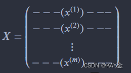
- 20 × 20的像素网格被“展开”成一个400维的向量。每个训练例子成为我们的数据矩阵 X 中的一行。
这给了我们一个1000x400矩阵 X,其中每一行是一个手写数字图像的训练例子。
训练集的第二部分是一个1000x1维向量 y,它包含训练集的标签。如果图像为数字0,则 y = 0; 如果图像为数字1,则 y = 1。
这是 MNIST 手写数字数据集( http://yann.lecun.com/exdb/MNIST/)的一个子集
# load dataset
X, y = load_data()
为了更加熟悉数据集。打印出每个变量,看看它包含什么。下面的代码打印变量 X 和 y 的元素。
print ('The first element of X is: ', X[0])输出:
The first element of X is:  [ 0.00000000e+00  0.00000000e+00  0.00000000e+00  0.00000000e+00
  0.00000000e+00  0.00000000e+00  0.00000000e+00  0.00000000e+00
  0.00000000e+00  0.00000000e+00  0.00000000e+00  0.00000000e+00
  0.00000000e+00  0.00000000e+00  0.00000000e+00  0.00000000e+00
  0.00000000e+00  0.00000000e+00  0.00000000e+00  0.00000000e+00
  0.00000000e+00  0.00000000e+00  0.00000000e+00  0.00000000e+00
  0.00000000e+00  0.00000000e+00  0.00000000e+00  0.00000000e+00
  0.00000000e+00  0.00000000e+00  0.00000000e+00  0.00000000e+00
  0.00000000e+00  0.00000000e+00  0.00000000e+00  0.00000000e+00
  0.00000000e+00  0.00000000e+00  0.00000000e+00  0.00000000e+00
  0.00000000e+00  0.00000000e+00  0.00000000e+00  0.00000000e+00
  0.00000000e+00  0.00000000e+00  0.00000000e+00  0.00000000e+00
  0.00000000e+00  0.00000000e+00  0.00000000e+00  0.00000000e+00
  0.00000000e+00  0.00000000e+00  0.00000000e+00  0.00000000e+00
  0.00000000e+00  0.00000000e+00  0.00000000e+00  0.00000000e+00
  0.00000000e+00  0.00000000e+00  0.00000000e+00  0.00000000e+00
  0.00000000e+00  0.00000000e+00  0.00000000e+00  8.56059680e-06
  1.94035948e-06 -7.37438725e-04 -8.13403799e-03 -1.86104473e-02
 -1.87412865e-02 -1.87572508e-02 -1.90963542e-02 -1.64039011e-02
 -3.78191381e-03  3.30347316e-04  1.27655229e-05  0.00000000e+00
  0.00000000e+00  0.00000000e+00  0.00000000e+00  0.00000000e+00
  0.00000000e+00  0.00000000e+00  1.16421569e-04  1.20052179e-04
 -1.40444581e-02 -2.84542484e-02  8.03826593e-02  2.66540339e-01
  2.73853746e-01  2.78729541e-01  2.74293607e-01  2.24676403e-01
  2.77562977e-02 -7.06315478e-03  2.34715414e-04  0.00000000e+00
  0.00000000e+00  0.00000000e+00  0.00000000e+00  0.00000000e+00
  0.00000000e+00  1.28335523e-17 -3.26286765e-04 -1.38651604e-02
  8.15651552e-02  3.82800381e-01  8.57849775e-01  1.00109761e+00
  9.69710638e-01  9.30928598e-01  1.00383757e+00  9.64157356e-01
  4.49256553e-01 -5.60408259e-03 -3.78319036e-03  0.00000000e+00
  0.00000000e+00  0.00000000e+00  0.00000000e+00  5.10620915e-06
  4.36410675e-04 -3.95509940e-03 -2.68537241e-02  1.00755014e-01
  6.42031710e-01  1.03136838e+00  8.50968614e-01  5.43122379e-01
  3.42599738e-01  2.68918777e-01  6.68374643e-01  1.01256958e+00
  9.03795598e-01  1.04481574e-01 -1.66424973e-02  0.00000000e+00
  0.00000000e+00  0.00000000e+00  0.00000000e+00  2.59875260e-05
 -3.10606987e-03  7.52456076e-03  1.77539831e-01  7.92890120e-01
  9.65626503e-01  4.63166079e-01  6.91720680e-02 -3.64100526e-03
 -4.12180405e-02 -5.01900656e-02  1.56102907e-01  9.01762651e-01
  1.04748346e+00  1.51055252e-01 -2.16044665e-02  0.00000000e+00
  0.00000000e+00  0.00000000e+00  5.87012352e-05 -6.40931373e-04
 -3.23305249e-02  2.78203465e-01  9.36720163e-01  1.04320956e+00
  5.98003217e-01 -3.59409041e-03 -2.16751770e-02 -4.81021923e-03
  6.16566793e-05 -1.23773318e-02  1.55477482e-01  9.14867477e-01
  9.20401348e-01  1.09173902e-01 -1.71058007e-02  0.00000000e+00
  0.00000000e+00  1.56250000e-04 -4.27724104e-04 -2.51466503e-02
  1.30532561e-01  7.81664862e-01  1.02836583e+00  7.57137601e-01
  2.84667194e-01  4.86865128e-03 -3.18688725e-03  0.00000000e+00
  8.36492601e-04 -3.70751123e-02  4.52644165e-01  1.03180133e+00
  5.39028101e-01 -2.43742611e-03 -4.80290033e-03  0.00000000e+00
  0.00000000e+00 -7.03635621e-04 -1.27262443e-02  1.61706648e-01
  7.79865383e-01  1.03676705e+00  8.04490400e-01  1.60586724e-01
 -1.38173339e-02  2.14879493e-03 -2.12622549e-04  2.04248366e-04
 -6.85907627e-03  4.31712963e-04  7.20680947e-01  8.48136063e-01
  1.51383408e-01 -2.28404366e-02  1.98971950e-04  0.00000000e+00
  0.00000000e+00 -9.40410539e-03  3.74520505e-02  6.94389110e-01
  1.02844844e+00  1.01648066e+00  8.80488426e-01  3.92123945e-01
 -1.74122413e-02 -1.20098039e-04  5.55215142e-05 -2.23907271e-03
 -2.76068376e-02  3.68645493e-01  9.36411169e-01  4.59006723e-01
 -4.24701797e-02  1.17356610e-03  1.88929739e-05  0.00000000e+00
  0.00000000e+00 -1.93511951e-02  1.29999794e-01  9.79821705e-01
  9.41862388e-01  7.75147704e-01  8.73632241e-01  2.12778350e-01
 -1.72353349e-02  0.00000000e+00  1.09937426e-03 -2.61793751e-02
  1.22872879e-01  8.30812662e-01  7.26501773e-01  5.24441863e-02
 -6.18971913e-03  0.00000000e+00  0.00000000e+00  0.00000000e+00
  0.00000000e+00 -9.36563862e-03  3.68349741e-02  6.99079299e-01
  1.00293583e+00  6.05704402e-01  3.27299224e-01 -3.22099249e-02
 -4.83053002e-02 -4.34069138e-02 -5.75151144e-02  9.55674190e-02
  7.26512627e-01  6.95366966e-01  1.47114481e-01 -1.20048679e-02
 -3.02798203e-04  0.00000000e+00  0.00000000e+00  0.00000000e+00
  0.00000000e+00 -6.76572712e-04 -6.51415556e-03  1.17339359e-01
  4.21948410e-01  9.93210937e-01  8.82013974e-01  7.45758734e-01
  7.23874268e-01  7.23341725e-01  7.20020340e-01  8.45324959e-01
  8.31859739e-01  6.88831870e-02 -2.77765012e-02  3.59136710e-04
  7.14869281e-05  0.00000000e+00  0.00000000e+00  0.00000000e+00
  0.00000000e+00  1.53186275e-04  3.17353553e-04 -2.29167177e-02
 -4.14402914e-03  3.87038450e-01  5.04583435e-01  7.74885876e-01
  9.90037446e-01  1.00769478e+00  1.00851440e+00  7.37905042e-01
  2.15455291e-01 -2.69624864e-02  1.32506127e-03  0.00000000e+00
  0.00000000e+00  0.00000000e+00  0.00000000e+00  0.00000000e+00
  0.00000000e+00  0.00000000e+00  0.00000000e+00  2.36366422e-04
 -2.26031454e-03 -2.51994485e-02 -3.73889910e-02  6.62121228e-02
  2.91134498e-01  3.23055726e-01  3.06260315e-01  8.76070942e-02
 -2.50581917e-02  2.37438725e-04  0.00000000e+00  0.00000000e+00
  0.00000000e+00  0.00000000e+00  0.00000000e+00  0.00000000e+00
  0.00000000e+00  0.00000000e+00  0.00000000e+00  0.00000000e+00
  0.00000000e+00  6.20939216e-18  6.72618320e-04 -1.13151411e-02
 -3.54641066e-02 -3.88214912e-02 -3.71077412e-02 -1.33524928e-02
  9.90964718e-04  4.89176960e-05  0.00000000e+00  0.00000000e+00
  0.00000000e+00  0.00000000e+00  0.00000000e+00  0.00000000e+00
  0.00000000e+00  0.00000000e+00  0.00000000e+00  0.00000000e+00
  0.00000000e+00  0.00000000e+00  0.00000000e+00  0.00000000e+00
  0.00000000e+00  0.00000000e+00  0.00000000e+00  0.00000000e+00
  0.00000000e+00  0.00000000e+00  0.00000000e+00  0.00000000e+00
  0.00000000e+00  0.00000000e+00  0.00000000e+00  0.00000000e+00
  0.00000000e+00  0.00000000e+00  0.00000000e+00  0.00000000e+00
  0.00000000e+00  0.00000000e+00  0.00000000e+00  0.00000000e+00
  0.00000000e+00  0.00000000e+00  0.00000000e+00  0.00000000e+00
  0.00000000e+00  0.00000000e+00  0.00000000e+00  0.00000000e+00
  0.00000000e+00  0.00000000e+00  0.00000000e+00  0.00000000e+00]
print ('The first element of y is: ', y[0,0])
print ('The last element of y is: ', y[-1,0])
输出:
The first element of y is:  0
The last element of y is:  1
熟悉数据的另一种方法是查看它的维度。请打印 X 和 y 的shape,并查看数据集中有多少训练示例。
print ('The shape of X is: ' + str(X.shape))
print ('The shape of y is: ' + str(y.shape))
输出:
The shape of X is: (1000, 400)
The shape of y is: (1000, 1)
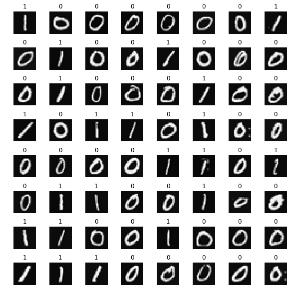
您将从可视化训练集的一个子集开始。
在下面的单元格中,代码从 X 中随机选择64行,将每行映射回20像素乘以20像素的灰度图像,并一起显示图像。每个图像的标签显示在图像的上方。
import warnings
warnings.simplefilter(action='ignore', category=FutureWarning)
# You do not need to modify anything in this cell

m, n = X.shape

fig, axes = plt.subplots(8,8, figsize=(8,8))
fig.tight_layout(pad=0.1)

for i,ax in enumerate(axes.flat):
    # Select random indices
    random_index = np.random.randint(m)

    # Select rows corresponding to the random indices and
    # reshape the image
    X_random_reshaped = X[random_index].reshape((20,20)).T

    # Display the image
    ax.imshow(X_random_reshaped, cmap='gray')

    # Display the label above the image
    ax.set_title(y[random_index,0])
    ax.set_axis_off()
输出:
2.2 模型展示
在此作业中使用的神经网络如下图所示。
它有三层、带激活函数。回想一下,输入是数字图像的像素值。因为图像的尺寸是20 × 20,给了400个输入。
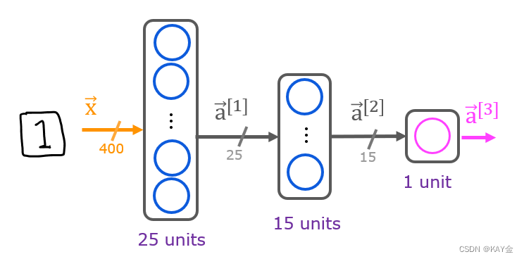
 这些参数的尺寸适用于第一层有25个单元的神经网络,第二层有15个单元,第三层有1个输出单元。回顾这些参数的尺寸确定如下:
如果网络在一个层中有 sin 单元,在下一个层中有 sout 单元,那么W 尺寸为 sin × sout,B 是一个带有 sout 元素的向量。
因此,W 和 b 的形状是
层1: W1的形状是(400,25) ,b1的形状是(25,)
层2: W2的形状是(25,15) ,而 b2的形状是: (15,)
层3: W3的形状是(15,1) ,b3的形状是: (1,)
2.3 Tensorflow模型实现
Tensorflow模型是一层一层地建立起来的。为您计算一个层的输入维度(上面的 sin)。您可以指定一个层的输出维度,这将决定下一个层的输入维度。第一层的输入维度来自于下面的 model.fit 语句中指定的输入数据的大小。
注意: 也可以添加一个输入层来指定第一层的输入维度。例如:
Keras. Input (form = (400,)) ,# 指定输入形状
下面,使用 Kera 序列模型和Dense Layer with a sigmoid activation来构建上述网络。
# UNQ_C1
# GRADED CELL: Sequential model


model = Sequential(
    [
        tf.keras.Input(shape=(400,)),    # specify input size (optional)
        Dense(25, activation='sigmoid'),
        Dense(15, activation='sigmoid'),
        Dense(1,  activation='sigmoid')
    ], name = "my_model"
)
model.summary()
输出:
Model: "my_model"
_________________________________________________________________
Layer (type)                 Output Shape              Param #
=================================================================
dense (Dense)                (None, 25)                10025
_________________________________________________________________
dense_1 (Dense)              (None, 15)                390
_________________________________________________________________
dense_2 (Dense)              (None, 1)                 16
=================================================================
Total params: 10,431
Trainable params: 10,431
Non-trainable params: 0
_________________________________________________________________
函数的作用是: 显示模型的有用摘要。由于我们已经指定了一个输入层大小,重量和偏置阵列的形状被确定,每层参数的总数可以显示。注意,层的名称可能会因为它们是自动生成的而有所不同。摘要中显示的参数计数与权重和偏置数组中的元素数量相对应,如下所示。
L1_num_params = 400 * 25 + 25  # W1 parameters  + b1 parameters
L2_num_params = 25 * 15 + 15   # W2 parameters  + b2 parameters
L3_num_params = 15 * 1 + 1     # W3 parameters  + b3 parameters
print("L1 params = ", L1_num_params, ", L2 params = ", L2_num_params, ",  L3 params = ", L3_num_params )
输出:
L1 params = 10025 , L2 params = 390 , L3 params = 16
下面的代码将定义一个损失函数并运行梯度下降法,以使模型的权重与训练数据相匹配。
model.compile(
    loss=tf.keras.losses.BinaryCrossentropy(),
    optimizer=tf.keras.optimizers.Adam(0.001),
)

model.fit(
    X,y,
    epochs=20
)

prediction = model.predict(X[0].reshape(1,400))  # a zero
print(f" predicting a zero: {prediction}")
prediction = model.predict(X[500].reshape(1,400))  # a one
print(f" predicting a one:  {prediction}")
模型的输出被解释为一个概率。在上面的第一个示例中,输入为零。该模型预测输入为1的概率接近于零。在第二个示例中,输入为1。该模型预测输入为1的概率接近于1。正如在逻辑回归的情况下,概率是比较一个门槛,以作出最后的预测。
import warnings
warnings.simplefilter(action='ignore', category=FutureWarning)
# You do not need to modify anything in this cell

m, n = X.shape

fig, axes = plt.subplots(8,8, figsize=(8,8))
fig.tight_layout(pad=0.1,rect=[0, 0.03, 1, 0.92]) #[left, bottom, right, top]

for i,ax in enumerate(axes.flat):
    # Select random indices
    random_index = np.random.randint(m)

    # Select rows corresponding to the random indices and
    # reshape the image
    X_random_reshaped = X[random_index].reshape((20,20)).T

    # Display the image
    ax.imshow(X_random_reshaped, cmap='gray')

    # Predict using the Neural Network
    prediction = model.predict(X[random_index].reshape(1,400))
    if prediction >= 0.5:
        yhat = 1
    else:
        yhat = 0

    # Display the label above the image
    ax.set_title(f"{y[random_index,0]},{yhat}")
    ax.set_axis_off()
fig.suptitle("Label, yhat", fontsize=16)
plt.show()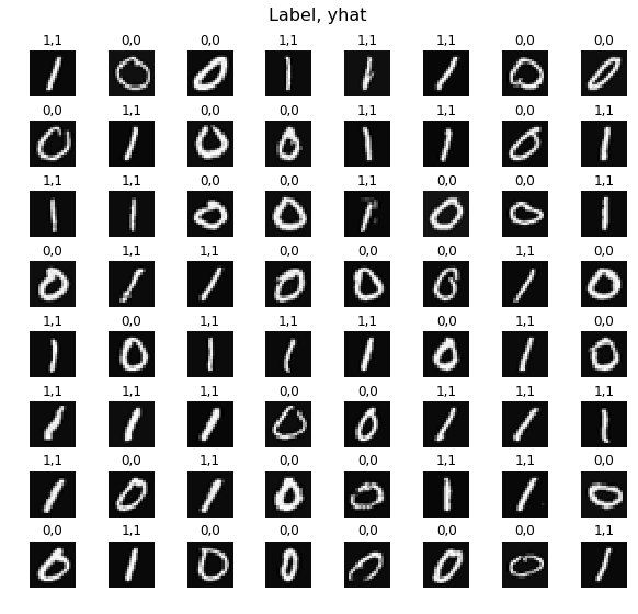


 386
386


 被折叠的 条评论
为什么被折叠?
被折叠的 条评论
为什么被折叠?
 到【灌水乐园】发言


