


一、程序及函数
1.引导脚本ex4.m
%% Machine Learning Online Class - Exercise 4 Neural Network Learning

%  Instructions
%  ------------------------------------------------------------------
%  This file contains code that helps you get started on the
%  linear exercise. You will need to complete the following functions
%  in this exericse:
%
%     sigmoidGradient.m
%     randInitializeWeights.m
%     nnCostFunction.m
%
%  For this exercise, you will not need to change any code in this file,
%  or any other files other than those mentioned above.

%% Initialization
clear;
close all;
clc

%% Setup the parameters you will use for this exercise
input_layer_size  = 400;  % 20x20 Input Images of Digits
hidden_layer_size = 25;   % 25 hidden units
num_labels = 10;          % 10 labels, from 1 to 10 (note that we have mapped "0" to label 10)

%% =========== Part 1: Loading and Visualizing Data =============
%  We start the exercise by first loading and visualizing the dataset.
%  You will be working with a dataset that contains handwritten digits.
%

% Load Training Data
fprintf('Loading and Visualizing Data ...\n')

load('ex4data1.mat');
m = size(X, 1);

% Randomly select 100 data points to display
% randperm生成1-5000的随机整数
sel = randperm(size(X, 1));
% 取sel的前100项
sel = sel(1:100);

displayData(X(sel, :));

fprintf('Program paused. Press enter to continue.\n');
pause;

%% ================ Part 2: Loading Parameters ================
% In this part of the exercise, we load some pre-initialized
% neural network parameters.

fprintf('\nLoading Saved Neural Network Parameters ...\n')

% Load the weights into variables Theta1 and Theta2
load('ex4weights.mat');

% Unroll parameters
nn_params = [Theta1(:); Theta2(:)];

%% ================ Part 3: Compute Cost (Feedforward) ================
%  To the neural network, you should first start by implementing the
%  feedforward part of the neural network that returns the cost only. You
%  should complete the code in nnCostFunction.m to return cost. After
%  implementing the feedforward to compute the cost, you can verify that
%  your implementation is correct by verifying that you get the same cost
%  as us for the fixed debugging parameters.
%
%  We suggest implementing the feedforward cost *without* regularization
%  first so that it will be easier for you to debug. Later, in part 4, you
%  will get to implement the regularized cost.
%
fprintf('\nFeedforward Using Neural Network ...\n')

% Weight regularization parameter (we set this to 0 here).
% 在Part3中我们先不用正则化
lambda = 0;

J = nnCostFunction(nn_params, input_layer_size, hidden_layer_size, ...
                   num_labels, X, y, lambda);

fprintf(['Cost at parameters (loaded from ex4weights): %f '...
         '\n(this value should be about 0.287629)\n'], J);

fprintf('\nProgram paused. Press enter to continue.\n');
pause;

%% =============== Part 4: Implement Regularization ===============
%  Once your cost function implementation is correct, you should now
%  continue to implement the regularization with the cost.

fprintf('\nChecking Cost Function (With Regularization) ... \n')

% Weight regularization parameter (we set this to 1 here).
lambda = 1;

J = nnCostFunction(nn_params, input_layer_size, hidden_layer_size, ...
                   num_labels, X, y, lambda);

fprintf(['Cost at parameters (loaded from ex4weights): %f '...
         '\n(this value should be about 0.383770)\n'], J);

fprintf('Program paused. Press enter to continue.\n');
pause;

%% ================ Part 5: Sigmoid Gradient  ================
%  Before you start implementing the neural network, you will first
%  implement the gradient for the sigmoid function. You should complete the
%  code in the sigmoidGradient.m file.

fprintf('\nEvaluating sigmoid gradient...\n')

g = sigmoidGradient([-1 -0.5 0 0.5 1]);
fprintf('Sigmoid gradient evaluated at [-1 -0.5 0 0.5 1]:\n  ');
fprintf('%f ', g);
fprintf('\n\n');

fprintf('Program paused. Press enter to continue.\n');
pause;

%% ================ Part 6: Initializing Pameters ================
%  In this part of the exercise, you will be starting to implment a two
%  layer neural network that classifies digits. You will start by
%  implementing a function to initialize the weights of the neural network
%  (randInitializeWeights.m)

fprintf('\nInitializing Neural Network Parameters ...\n')

initial_Theta1 = randInitializeWeights(input_layer_size, hidden_layer_size);
initial_Theta2 = randInitializeWeights(hidden_layer_size, num_labels);

% Unroll parameters
initial_nn_params = [initial_Theta1(:) ; initial_Theta2(:)];

%% =============== Part 7: Implement Backpropagation ===============
%  Once your cost matches up with ours, you should proceed to implement the
%  backpropagation algorithm for the neural network. You should add to the
%  code you've written in nnCostFunction.m to return the partial
%  derivatives of the parameters.
%
fprintf('\nChecking Backpropagation... \n');

%  Check gradients by running checkNNGradients
% 检查我们之前写的梯度计算函数有没有问题
checkNNGradients;

fprintf('\nProgram paused. Press enter to continue.\n');
pause;

%% =============== Part 8: Implement Regularization ===============
%  Once your backpropagation implementation is correct, you should now
%  continue to implement the regularization with the cost and gradient.

fprintf('\nChecking Backpropagation (w/ Regularization) ... \n')

%  Check gradients by running checkNNGradients
lambda = 3;
checkNNGradients(lambda);

% Also output the costFunction debugging values
debug_J  = nnCostFunction(nn_params, input_layer_size, ...
                          hidden_layer_size, num_labels, X, y, lambda);

fprintf(['\n\nCost at (fixed) debugging parameters (w/ lambda = %f): %f ' ...
         '\n(for lambda = 3, this value should be about 0.576051)\n\n'], lambda, debug_J);

fprintf('Program paused. Press enter to continue.\n');
pause;

%% =================== Part 8: Training NN ===================
%  You have now implemented all the code necessary to train a neural
%  network. To train your neural network, we will now use "fmincg", which
%  is a function which works similarly to "fminunc". Recall that these
%  advanced optimizers are able to train our cost functions efficiently as
%  long as we provide them with the gradient computations.
%
fprintf('\nTraining Neural Network... \n')
% 开始计时
tic;
%  After you have completed the assignment, change the MaxIter to a larger
%  value to see how more training helps.
options = optimset('MaxIter', 50);

%  You should also try different values of lambda
lambda = 1;

% Create "short hand" for the cost function to be minimized
costFunction = @(p) nnCostFunction(p, ...
                                   input_layer_size, ...
                                   hidden_layer_size, ...
                                   num_labels, X, y, lambda);

% Now, costFunction is a function that takes in only one argument (the
% neural network parameters)
[nn_params, cost] = fmincg(costFunction, initial_nn_params, options);

% Obtain Theta1 and Theta2 back from nn_params
Theta1 = reshape(nn_params(1:hidden_layer_size * (input_layer_size + 1)), ...
                 hidden_layer_size, (input_layer_size + 1));

Theta2 = reshape(nn_params((1 + (hidden_layer_size * (input_layer_size + 1))):end), ...
                 num_labels, (hidden_layer_size + 1));
% 计时结束输出本次训练时间
toc;
fprintf('Program paused. Press enter to continue.\n');
pause;

%% ================= Part 9: Visualize Weights =================
%  You can now "visualize" what the neural network is learning by
%  displaying the hidden units to see what features they are capturing in
%  the data.

fprintf('\nVisualizing Neural Network... \n')

displayData(Theta1(:, 2:end));

fprintf('\nProgram paused. Press enter to continue.\n');
pause;

%% ================= Part 10: Implement Predict =================
%  After training the neural network, we would like to use it to predict
%  the labels. You will now implement the "predict" function to use the
%  neural network to predict the labels of the training set. This lets
%  you compute the training set accuracy.

pred = predict(Theta1, Theta2, X);

fprintf('\nTraining Set Accuracy: %f\n', mean(double(pred == y)) * 100);
2.核心函数 nnCostFunction.m
这是BP神经网络最核心的东西,基本上重要的语句我都写了注释。
感觉只要细心一点,搞清楚每个向量和矩阵的尺寸就没啥问题了。
function [J grad] = nnCostFunction(nn_params, ...
                                   input_layer_size, ...
                                   hidden_layer_size, ...
                                   num_labels, ...
                                   X, y, lambda)
%NNCOSTFUNCTION Implements the neural network cost function for a two layer
%neural network which performs classification
%   [J grad] = NNCOSTFUNCTON(nn_params, hidden_layer_size, num_labels, ...
%   X, y, lambda) computes the cost and gradient of the neural network. The
%   parameters for the neural network are "unrolled" into the vector
%   nn_params and need to be converted back into the weight matrices.
%
%   The returned parameter grad should be a "unrolled" vector of the
%   partial derivatives of the neural network.
%

% Reshape nn_params back into the parameters Theta1 and Theta2, the weight matrices
% for our 2 layer neural network
Theta1 = reshape(nn_params(1:hidden_layer_size * (input_layer_size + 1)), ...
                 hidden_layer_size, (input_layer_size + 1));

Theta2 = reshape(nn_params((1 + (hidden_layer_size * (input_layer_size + 1))):end), ...
                 num_labels, (hidden_layer_size + 1));

% Setup some useful variables
m = size(X, 1);

% You need to return the following variables correctly

% ====================== YOUR CODE HERE ======================
% Instructions: You should complete the code by working through the
%               following parts.
%
% Part 1: Feedforward the neural network and return the cost in the
%         variable J. After implementing Part 1, you can verify that your
%         cost function computation is correct by verifying the cost
%         computed in ex4.m
%
% Part 2: Implement the backpropagation algorithm to compute the gradients
%         Theta1_grad and Theta2_grad. You should return the partial derivatives of
%         the cost function with respect to Theta1 and Theta2 in Theta1_grad and
%         Theta2_grad, respectively. After implementing Part 2, you can check
%         that your implementation is correct by running checkNNGradients
%
%         Note: The vector y passed into the function is a vector of labels
%               containing values from 1..K. You need to map this vector into a
%               binary vector of 1's and 0's to be used with the neural network
%               cost function.
%
%         Hint: We recommend implementing backpropagation using a for-loop
%               over the training examples if you are implementing it for the
%               first time.
%
% Part 3: Implement regularization with the cost function and gradients.
%
%         Hint: You can implement this around the code for
%               backpropagation. That is, you can compute the gradients for
%               the regularization separately and then add them to Theta1_grad
%               and Theta2_grad from Part 2.
%
% 初始化部分
% Add ones to the X data matrix
X = [ones(m, 1) X];
% 初始化sum1为外层循环的累加和,最后乘上1/m得到J值
sum1 = 0;
% 初始化输出层和隐含层的反向传播误差delta_3,delta_2
delta_3 = zeros(num_labels,1);
delta_2 = zeros(hidden_layer_size + 1,1);
% 初始化两个权重矩阵真正的偏导数矩阵
Theta1_grad = zeros(size(Theta1));
Theta2_grad = zeros(size(Theta2));

% 正式计算部分
% 处理每一个样本
for i = 1 : m
    % temp_a1是当前输入,尺寸为401×1
    temp_a1 = X(i,:)';
    temp_z2 = Theta1 * temp_a1;
    % 给隐含层添加一个偏置,值为1
    temp_z2 = [1;temp_z2];
    % temp_a2是当前隐含层输出,尺寸为26×1
    temp_a2 = sigmoid(temp_z2);
    % temp_z3是当前输出层输入,尺寸为10×1
    temp_z3 = Theta2 * temp_a2;
    % temp_a3是当前输出层输出,尺寸为10×1
    temp_a3 = sigmoid(temp_z3);
    % 初始化当前样本的输出层理论值为全0
    y_temp = zeros(num_labels,1);
    % 如果当前样本是数字y(i),则y_temp(y(i))=1,其余为0
    y_temp(y(i)) = 1;
    % 计算delta_3,尺寸为10×1
    delta_3 = temp_a3 - y_temp;
    % 计算delta_2,尺寸为26×1
    delta_2 = (Theta2' * delta_3) .* sigmoidGradient(temp_z2);
    % 应舍弃delta_2(1)。若不舍弃,将导致隐含层偏置项被计算出一个值
    %(而实际上这个偏置值为1的项是我们人为加上去的,并不是算出来的)
    delta_2 = delta_2(2:end);
    Theta2_grad = Theta2_grad + delta_3 * temp_a2';
    Theta1_grad = Theta1_grad + delta_2 * temp_a1';

    %初始化sum2为当前内层循环的累加和
    sum2 = 0;
    for k = 1 : num_labels
        sum2 = sum2 + ( -1 .* y_temp(k) .* log(temp_a3(k)) - (1 - y_temp(k)) .* log(1 - temp_a3(k)) );
    end
    sum1 = sum1 + sum2;
end

% 开始计算正则化项值
% 取Theta1和Theta2的第二列到最后一列,因为它们的第一列和偏置项有关
Theta1_temp = Theta1(:,2:end);
Theta2_temp = Theta2(:,2:end);
% 计算Theta1,Theta2各自的元素平方和
sum_Theta1_temp = sum(Theta1_temp(:).^2);
sum_Theta2_temp = sum(Theta2_temp(:).^2);

% 计算带有正则化项的J值
J = 1 ./ m .* sum1 + lambda / (2 * m) * (sum_Theta1_temp + sum_Theta2_temp);

% 最终得到J对于Theta1,Theta2中各元素的偏导数值
% 注意:和偏置项有关的两个矩阵的第一列不加正则化项,其余列都要加上正则化项
% 先求权重矩阵1的第一列
Theta1_grad(:,1) = 1 / m * Theta1_grad(:,1);
% 再求权重矩阵1的第二列到最后一列
Theta1_grad(:,2:end) = 1 / m * Theta1_grad(:,2:end) + lambda / m * Theta1(:,2:end);
% 先求权重矩阵2的第一列
Theta2_grad(:,1) = 1 / m * Theta2_grad(:,1);
% 再求权重矩阵2的第二列到最后一列
Theta2_grad(:,2:end) = 1 / m * Theta2_grad(:,2:end) + lambda / m * Theta2(:,2:end);
% =========================================================================

% Unroll gradients
grad = [Theta1_grad(:) ; Theta2_grad(:)];

end
3.sigmoidGradient.m
function g = sigmoidGradient(z)
%SIGMOIDGRADIENT returns the gradient of the sigmoid function
%evaluated at z
%   g = SIGMOIDGRADIENT(z) computes the gradient of the sigmoid function
%   evaluated at z. This should work regardless if z is a matrix or a
%   vector. In particular, if z is a vector or matrix, you should return
%   the gradient for each element.

g = zeros(size(z));

% ====================== YOUR CODE HERE ======================
% Instructions: Compute the gradient of the sigmoid function evaluated at
%               each value of z (z can be a matrix, vector or scalar).

g = sigmoid(z) .* (1 - sigmoid(z));

% =============================================================

end
4.computeNumericalGradient.m
这个函数的功能是用数值化的方法给出J对每个权重的偏导值,用来验证我们自己写的求梯度的函数结果是否正确。
function numgrad = computeNumericalGradient(J, theta)
%COMPUTENUMERICALGRADIENT Computes the gradient using "finite differences"
%and gives us a numerical estimate of the gradient.
%   numgrad = COMPUTENUMERICALGRADIENT(J, theta) computes the numerical
%   gradient of the function J around theta. Calling y = J(theta) should
%   return the function value at theta.

% Notes: The following code implements numerical gradient checking, and
%        returns the numerical gradient.It sets numgrad(i) to (a numerical
%        approximation of) the partial derivative of J with respect to the
%        i-th input argument, evaluated at theta. (i.e., numgrad(i) should
%        be the (approximately) the partial derivative of J with respect
%        to theta(i).)
%

% numgrad是要检验的theta元素的总个数
numgrad = zeros(size(theta));
% perturb是要加/减在theta长列向量上的小量
perturb = zeros(size(theta));
e = 1e-4;
for p = 1:numel(theta)
    % Set perturbation vector
    % 对于第i个元素,设置perturb的第i个元素为小量e,其余均为0
    perturb(p) = e;
    % 计算J(theta+)和(theta-)
    loss1 = J(theta - perturb);
    loss2 = J(theta + perturb);
    % 计算数值化的梯度
    numgrad(p) = (loss2 - loss1) / (2*e);
    % 处理完第i个元素后,重新置perturb的第i个元素为0
    perturb(p) = 0;
end
end
其他函数都是Andrew Ng已经帮我们写好了的,相对不那么重要,就不贴上来了。
二、运行结果
执行ex4.m,一开始的输出结果就是一些基本值的校验过程,用来检验你写的函数是不是对的。

将一些测试样本图像可视化一下:

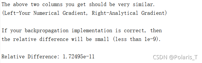
下图是在我们用函数计算出的theta梯度解析解和数值化theta梯度间进行比较,可以发现它们俩之间误差很小,足以证明我们函数写的是正确无误的。
这是最优化J值的过程(迭代50次/100次),可以发现当lambda值较小而迭代次数较多时,总训练时间会变得贼慢。。。


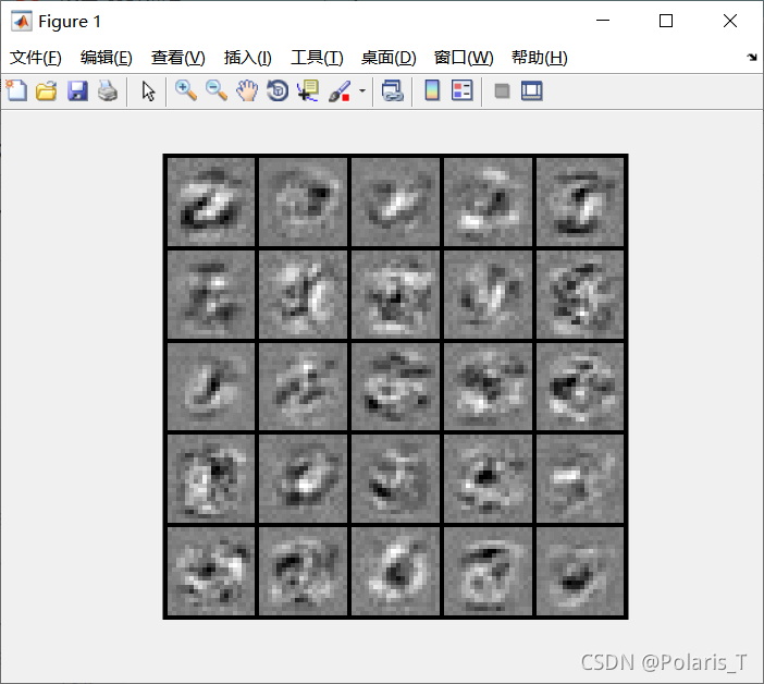
将隐含层“学习”到的东西可视化一下(当然这玩意儿不具备可解释性,反正人类肯定看不懂。。。):
最后得出用训练好的神经网络预测5000个测试样本的正确率为95.32%(lambda = 1,迭代次数为50)。

lambda = 0.05,迭代次数为100时可以看到准确率接近100%,但这不是什么好事,因为我们调低了lambda会导致正则化项很小从而使得网络更倾向于减小J值,最终可能发生过拟合现象,使得神经网络泛化能力降低,所以我们在实际训练神经网络的过程中,要找到一个较为平衡的lambda值。


 460
460


 被折叠的 条评论
为什么被折叠?
被折叠的 条评论
为什么被折叠?
 到【灌水乐园】发言


