


In[1]:
import random
import numpy as np
from cs231n.data_utils import load_CIFAR10
import matplotlib.pyplot as plt
from __future__ import print_function
#%matplotlib inline  如果是jupyterbook你就使用该语句,如果是ipython你就不适用
# figsize设置图形大小,宽10.0,高8.0, interpolation是图像内插 cmap是分配颜色
plt.rcParams['figure.figsize'] = (10.0, 8.0)
plt.rcParams['image.interpolation'] = 'nearest'
plt.rcParams['image.cmap'] = 'gray'
%load_ext autoreload
%autoreload 2
# %load_ext autoreload在执行用户代码前,重新装入 软件的扩展和模块
# autoreload 意思是自动重新装入,0:不执行装入命令 1:只装入%aimport要装入的模块 2:装入所有aimport不包含的模块
In[2]:
载入数据
# Load the raw CIFAR-10 data.
cifar10_dir = 'cs231n/datasets/cifar-10-batches-py'

# Cleaning up variables to prevent loading data multiple times (which may cause memory issue)
try:
   del X_train, y_train
   del X_test, y_test
   print('Clear previously loaded data.')
except:
   pass

X_train, y_train, X_test, y_test = load_CIFAR10(cifar10_dir)

# As a sanity check, we print out the size of the training and test data.
print('Training data shape: ', X_train.shape)
print('Training labels shape: ', y_train.shape)
print('Test data shape: ', X_test.shape)
print('Test labels shape: ', y_test.shape)

In[3]:
可视化数据
import matplotlib as mpl
mpl.use('TkAgg')
# 类(labels)
classes = ['plane', 'car', 'bird', 'cat', 'deer', 'dog', 'frog', 'horse', 'ship', 'truck']
num_classes = len(classes)
#每个类别采样数
samples_per_class = 7
# cls代指类
#enumerate 枚举 (0,plane 1,car 2,bird……)
for y, cls in enumerate(classes):
    #找出矩阵中非零元素y_train=y的位置
	idxs = np.flatnonzero(y_train == y)
# 在idxs中选出samples_per_class个样本,replace:false表示不能取相同数字
    idxs = np.random.choice(idxs, samples_per_class, replace=False)
# 随机从对所选的样本的位置和样本所对应的图片在训练集中的位置进行循环
for i, idx in enumerate(idxs):
        plt_idx = i * num_classes + y + 1 #分别对应的类
        plt.subplot(samples_per_class, num_classes, plt_idx) #参数1代表行数、参数2代表列数、参数3代表第几个图,之所以每次都需要输入第1、2个参数,这两个参数是可变的
        plt.imshow(X_train[idx].astype('uint8'))#画图, plt.imshow(a)中a的格式要求是width*height*depth,数据类型是无符号整型(uint8),由上一个函数指定宽高深
        plt.axis('off') #关闭坐标轴
        if i == 0:
            plt.title(cls) #写上类别名
plt.show()#显示

In[4]:
将数据分割为train, val和test集。此外,我们会创建一个小的开发集作为培训数据的子集; 我们可以在开发中使用它,这样我们的代码运行得更快。
num_training = 49000
num_validation = 1000
num_test = 1000
num_dev = 500

mask = range(num_training, num_training + num_validation)
X_val = X_train[mask]
y_val = y_train[mask]

mask = range(num_training)
X_train = X_train[mask]
y_train = y_train[mask]


mask = np.random.choice(num_training, num_dev, replace=False) #在num_training中随机挑出不重复的num_dev
X_dev = X_train[mask]
y_dev = y_train[mask]

mask = range(num_test)
X_test = X_test[mask]
y_test = y_test[mask]

print('Train data shape: ', X_train.shape)
print('Train labels shape: ', y_train.shape)
print('Validation data shape: ', X_val.shape)
print('Validation labels shape: ', y_val.shape)
print('Test data shape: ', X_test.shape)
print('Test labels shape: ', y_test.shape)

In[5]:
X_train = np.reshape(X_train, (X_train.shape[0], -1)) #这里将后面的维度合并
X_val = np.reshape(X_val, (X_val.shape[0], -1))
X_test = np.reshape(X_test, (X_test.shape[0], -1))
X_dev = np.reshape(X_dev, (X_dev.shape[0], -1))

print('Training data shape: ', X_train.shape)
print('Validation data shape: ', X_val.shape)
print('Test data shape: ', X_test.shape)
print('dev data shape: ', X_dev.shape)

In[6]:
预处理:均值得到图像
mean_image = np.mean(X_train, axis=0)# 压缩行,对各列求均值 得到图片在每个类的平均分数
print(mean_image[:10])
plt.figure(figsize=(4,4))
plt.imshow(mean_image.reshape((32,32,3)).astype('uint8'))
plt.show()

In[7]:
减去平均值
X_train -= mean_image
X_val -= mean_image
X_test -= mean_image
X_dev -= mean_image
ln[8]:
添加维度偏差
#np.hstack 沿着水平方向将数组堆叠起来。
X_train = np.hstack([X_train, np.ones((X_train.shape[0], 1))])  #将wx+b中的w和b合并
X_val = np.hstack([X_val, np.ones((X_val.shape[0], 1))])
X_test = np.hstack([X_test, np.ones((X_test.shape[0], 1))])
X_dev = np.hstack([X_dev, np.ones((X_dev.shape[0], 1))])
print(X_train.shape, X_val.shape, X_test.shape, X_dev.shape)

接下来填写linear_svm.py中的svm_loss_naive函数片段
from builtins import range
import numpy as np
from random import shuffle
from past.builtins import xrange


def svm_loss_naive(W, X, y, reg):
    """
    Structured SVM loss function, naive implementation (with loops).

    Inputs have dimension D, there are C classes, and we operate on minibatches
    of N examples.

    Inputs:
    - W: A numpy array of shape (D, C) containing weights. D is 32x32x3
    - X: A numpy array of shape (N, D) containing a minibatch of data.
    - y: A numpy array of shape (N,) containing training labels; y[i] = c means
      that X[i] has label c, where 0 <= c < C.
    - reg: (float) regularization strength

    Returns a tuple of:
    - loss as single float
    - gradient with respect to weights W; an array of same shape as W
    """
    dW = np.zeros(W.shape)  # initialize the gradient as zero

    # compute the loss and the gradient
    num_classes = W.shape[1]
    num_train = X.shape[0]
    loss = 0.0
    for i in range(num_train):
        scores = X[i].dot(W)
        correct_class_score = scores[y[i]]
        for j in range(num_classes):
            if j == y[i]:
                continue
            margin = scores[j] - correct_class_score + 1  # note delta = 1
            if margin > 0:
                dW[:, y[i]] = dW[:, y[i]] - X[i]
                dW[:, j] = dW[:, j] + X[i]
                loss += margin

    # Right now the loss is a sum over all training examples, but we want it
    # to be an average instead so we divide by num_train.
    loss /= num_train

    # Add regularization to the loss.
    loss += reg * np.sum(W * W)

    #############################################################################
    # TODO:                                                                     #
    # Compute the gradient of the loss function and store it dW.                #
    # Rather that first computing the loss and then computing the derivative,   #
    # it may be simpler to compute the derivative at the same time that the     #
    # loss is being computed. As a result you may need to modify some of the    #
    # code above to compute the gradient.                                       #
    #############################################################################
    # *****START OF YOUR CODE (DO NOT DELETE/MODIFY THIS LINE)*****

    dW /= num_train
    dW = dW + reg * 2 * W


    # *****END OF YOUR CODE (DO NOT DELETE/MODIFY THIS LINE)*****

    return loss, dW
In[9]:
估计损失函数
from cs231n.classifiers.linear_svm import svm_loss_naive
import time

# generate a random SVM weight matrix of small numbers
W = np.random.randn(3073, 10) * 0.0001

loss, grad = svm_loss_naive(W, X_dev, y_dev, 0.000005)
print('loss: %f' % (loss, ))

为了检查是否正确地实现了梯度,可以从数值上估计损失函数的梯度,并将数值估计与计算的梯度进行比较。我们已经为您提供了这样的代码:
ln[10]:
#计算W和损失的梯度
loss, grad = svm_loss_naive(W, X_dev, y_dev, 0.0)
#数值计算梯度沿着几个随机选择的维度, 将它们与解析计算的梯度进行比较
from cs231n.gradient_check import grad_check_sparse
f = lambda w: svm_loss_naive(w, X_dev, y_dev, 0.0)[0]# lambda 函数是一种小的匿名函数。
grad_numerical = grad_check_sparse(f, W, grad)
#正则化
loss, grad = svm_loss_naive(W, X_dev, y_dev, 5e1)
f = lambda w: svm_loss_naive(w, X_dev, y_dev, 5e1)[0]
grad_numerical = grad_check_sparse(f, W, grad)

内联问题1:
有时候gradcheck中的维度可能不完全匹配。这种差异是由什么引起的呢?这是值得担忧的原因吗?在一维中,梯度检查可能失败的简单例子是什么?如何改变发生频率的边际效应?提示:严格来说,SVM损失函数并不是可微的
你的回答:有可能gradcheck中的一个维度不完全匹配。让我们回忆一下SVM损失函数:max(0,x),其中x是错误类和正确类的分数之差加上一个常数。如果x > 0,那么我们会招致一些错误,否则,如果x < 0,我们将其阈值设为0。max函数的问题是当我们试图计算梯度时。一般来说,当我们有max(x,y)和x=y时,梯度是没有定义的,这些不可微的部分被称为扭结,它们是导致梯度检查失败的原因。作为一个简单的例子,如果x=-1e-8,那么max(0,x)=0,解析梯度是0;然而,如果我们考虑h大于x,数值梯度可能会不同,例如,h=1e-6。它将不同,因为当我们计算f(x+h) = max(0,x+h) = c > 0,因此数值梯度将不同于0。为了避免这个问题的出现频率,我们可以在计算梯度时考虑少量的数据点,因为数据点越少,我们的纠结就越少。另一种通常用于计算梯度的方法是次梯度。
svm_loss_vectorized函数
def svm_loss_vectorized(W, X, y, reg):
  """
  Structured SVM loss function, vectorized implementation.
  Inputs and outputs are the same as svm_loss_naive.
  """
  loss = 0.0
  dW = np.zeros(W.shape) # initialize the gradient as zero

  #############################################################################
  # TODO:                                                                     #
  # Implement a vectorized version of the structured SVM loss, storing the    #
  # result in loss.                                                           #
  #############################################################################
  # Compute the loss
  num_classes = W.shape[1]
  num_train = X.shape[0]
  scores = X.dot(W)
  correct_class_scores = scores[ np.arange(num_train), y].reshape(num_train,1)
  margin = np.maximum(0, scores - correct_class_scores + 1)
  margin[ np.arange(num_train), y] = 0 # do not consider correct class in loss
  loss = margin.sum() / num_train

  # Add regularization to the loss.
  loss += reg * np.sum(W * W)

  #############################################################################
  #                             END OF YOUR CODE                              #
  #############################################################################


  #############################################################################
  # TODO:                                                                     #
  # Implement a vectorized version of the gradient for the structured SVM     #
  # loss, storing the result in dW.                                           #
  #                                                                           #
  # Hint: Instead of computing the gradient from scratch, it may be easier    #
  # to reuse some of the intermediate values that you used to compute the     #
  # loss.                                                                     #
  #############################################################################
  # Compute gradient
  margin[margin > 0] = 1
  valid_margin_count = margin.sum(axis=1)
  # Subtract in correct class (-s_y)
  margin[np.arange(num_train),y ] -= valid_margin_count
  dW = (X.T).dot(margin) / num_train

  # Regularization gradient
  dW = dW + reg * 2 * W
  #############################################################################
  #                             END OF YOUR CODE                              #
  #############################################################################

  return loss, dW
In[11]:
比较矢量化和常规的区别
tic = time.time()
loss_naive, grad_naive = svm_loss_naive(W, X_dev, y_dev, 0.000005)
toc = time.time()
print('Naive loss: %e computed in %fs' % (loss_naive, toc - tic))

from cs231n.classifiers.linear_svm import svm_loss_vectorized
tic = time.time()
loss_vectorized, _ = svm_loss_vectorized(W, X_dev, y_dev, 0.000005)
toc = time.time()
print('Vectorized loss: %e computed in %fs' % (loss_vectorized, toc - tic))
print('difference: %f' % (loss_naive - loss_vectorized))

In[12]:
增加了梯度后的矢量化的差别
# Complete the implementation of svm_loss_vectorized, and compute the gradient
# of the loss function in a vectorized way.

# The naive implementation and the vectorized implementation should match, but
# the vectorized version should still be much faster.
tic = time.time()
_, grad_naive = svm_loss_naive(W, X_dev, y_dev, 0.000005)
toc = time.time()
print('Naive loss and gradient: computed in %fs' % (toc - tic))

tic = time.time()
_, grad_vectorized = svm_loss_vectorized(W, X_dev, y_dev, 0.000005)
toc = time.time()
print('Vectorized loss and gradient: computed in %fs' % (toc - tic))

# The loss is a single number, so it is easy to compare the values computed
# by the two implementations. The gradient on the other hand is a matrix, so
# we use the Frobenius norm to compare them.
difference = np.linalg.norm(grad_naive - grad_vectorized, ord='fro')
print('difference: %f' % difference)

Stochastic Gradient Descent(随机梯度下降法)
填写linear_classifier.py
from __future__ import print_function

import numpy as np
from cs231n.classifiers.linear_svm import *
from cs231n.classifiers.softmax import *


class LinearClassifier(object):

    def __init__(self):
        self.W = None

    def train(self, X, y, learning_rate=1e-3, reg=1e-5, num_iters=100,
              batch_size=200, verbose=False):
        """
        Train this linear classifier using stochastic gradient descent.

        Inputs:
        - X: 一个numpy数组的形状(N, D)包含训练数据;有N个每个维度D的训练样本。
        - y: 形状(N,)的numpy数组,包含训练标签;y[i]=c,表示X[i]对于c类有标号0<=c<C
        - learning_rate: (float) 学习率,用于优化
        - reg: (float) 正规化强度
        - num_iters: (integer) 优化时所采取的步骤数
        - batch_size: (integer) 每个步骤使用的训练示例的数量
        - verbose: (boolean) 如果为true,在优化过程中打印progress
        Outputs:
        在每个训练集迭代中包含损失函数值
        """
        num_train, dim = X.shape
        num_classes = np.max(y) + 1  # 假设y的值为0…K-1, K是类的数量
        if self.W is None:
            # 延迟初始化W
            self.W = 0.001 * np.random.randn(dim, num_classes)

        # 运行随机梯度下降来优化W
        loss_history = []
        for it in range(num_iters):
            X_batch = None
            y_batch = None

            #########################################################################
            # TODO:                                                                 #
            # Sample batch_size elements from the training data and their           #
            # corresponding labels to use in this round of gradient descent.        #
            # Store the data in X_batch and their corresponding labels in           #
            # y_batch; after sampling X_batch should have shape (dim, batch_size)   #
            # and y_batch should have shape (batch_size,)                           #
            #                                                                       #
            # Hint: Use np.random.choice to generate indices. Sampling with         #
            # replacement is faster than sampling without replacement.              #
            #########################################################################
            batch_indices = np.random.choice(num_train, batch_size, replace=False)
            X_batch = X[batch_indices]
            y_batch = y[batch_indices]
            #########################################################################
            #                       END OF YOUR CODE                                #
            #########################################################################

            # evaluate loss and gradient
            loss, grad = self.loss(X_batch, y_batch, reg)
            loss_history.append(loss)

            # perform parameter update
            #########################################################################
            # TODO:                                                                 #
            # Update the weights using the gradient and the learning rate.          #
            #########################################################################
            self.W = self.W - learning_rate * grad
            #########################################################################
            #                       END OF YOUR CODE                                #
            #########################################################################

            if verbose and it % 100 == 0:
                print('iteration %d / %d: loss %f' % (it, num_iters, loss))

        return loss_history

    def predict(self, X):
        """
        使用这个线性分类器训练的权值来预测数据点
        Inputs:
        - X:一个numpy数组的形状(N, D)包含训练数据;有N个每个维度D的训练样本。
        Returns:
        - y_pred:  x中数据的预测标签。y_pred是一维的数组的长度N,每个元素是一个整数给出预测类。
        """
        y_pred = np.zeros(X.shape[0])
        ###########################################################################
        # TODO:                                                                   #
        # Implement this method. Store the predicted labels in y_pred.            #
        ###########################################################################
        scores = X.dot(self.W)
        y_pred = scores.argmax(axis=1)
        ###########################################################################
        #                           END OF YOUR CODE                              #
        ###########################################################################
        return y_pred

    def loss(self, X_batch, y_batch, reg):
        """
        计算损失函数及其导数。
		子类会覆盖这个方法
        Inputs:
        - X_batch: 一个形状(N, D)的numpy数组,包含N个数据点的小批量;每个点的尺寸都是D
        - y_batch: 形状(N,)的numpy数组,包含minibatch的标签
        - reg: (float) 正则化

        Returns: 一个元组,其中包含:
        - 损失作为单一浮动
        - 关于self.W的梯度;与W形状相同的数组
        """
        pass


class LinearSVM(LinearClassifier):
    """ A subclass that uses the Multiclass SVM loss function """

    def loss(self, X_batch, y_batch, reg):
        return svm_loss_vectorized(self.W, X_batch, y_batch, reg)
In[13]:
from cs231n.classifiers import LinearSVM
svm = LinearSVM()
tic = time.time()
loss_hist = svm.train(X_train, y_train, learning_rate=1e-7, reg=2.5e4,
                      num_iters=1500, verbose=True)
toc = time.time()
print('That took %fs' % (toc - tic))

In[14]:
绘制损失函数图像
plt.plot(loss_hist)
plt.xlabel('Iteration number')
plt.ylabel('Loss value')
plt.show()

In[15]:
完成predict函数
y_train_pred = svm.predict(X_train)
print('training accuracy: %f' % (np.mean(y_train == y_train_pred), ))
y_val_pred = svm.predict(X_val)
print('validation accuracy: %f' % (np.mean(y_val == y_val_pred), ))

In[16]:
使用验证集来优化超参数(正则化强度和学习率)
learning_rates = [1e-7, 1e-6]
regularization_strengths = [2e4, 2.5e4, 3e4, 3.5e4, 4e4, 4.5e4, 5e4, 6e4]
# results是(learning_rate, regularization_strength)到(training_accuracy, validation_accuracy)的字典映射元组,准确性仅仅是被正确分类的数据点的一部分。
results = {}
best_val = -1   # 这是迄今为止我们所见过的最高验证精度。
best_svm = None # 线性支持向量机对象获得最高的验证率。
################################################################################
# TODO:                                                                        #
# Write code that chooses the best hyperparameters by tuning on the validation #
# set. For each combination of hyperparameters, train a linear SVM on the      #
# training set, compute its accuracy on the training and validation sets, and  #
# store these numbers in the results dictionary. In addition, store the best   #
# validation accuracy in best_val and the LinearSVM object that achieves this  #
# accuracy in best_svm.                                                        #
#                                                                              #
# Hint: You should use a small value for num_iters as you develop your         #
# validation code so that the SVMs don't take much time to train; once you are #
# confident that your validation code works, you should rerun the validation   #
# code with a larger value for num_iters.                                      #
################################################################################
# Obtain all possible combinations
grid_search = [ (lr,rg) for lr in learning_rates for rg in regularization_strengths ]

for lr, rg in grid_search:
    # Create a new SVM instance
    svm = LinearSVM()
    # Train the model with current parameters
    train_loss = svm.train(X_train, y_train, learning_rate=lr, reg=rg,
                      num_iters=1500, verbose=False)
    # Predict values for training set
    y_train_pred = svm.predict(X_train)
    # Calculate accuracy
    train_accuracy = np.mean(y_train_pred == y_train)
    # Predict values for validation set
    y_val_pred = svm.predict(X_val)
    # Calculate accuracy
    val_accuracy = np.mean(y_val_pred == y_val)
    # Save results
    results[(lr,rg)] = (train_accuracy, val_accuracy)
    if best_val < val_accuracy:
        best_val = val_accuracy
        best_svm = svm

################################################################################
#                              END OF YOUR CODE                                #
################################################################################

# Print out results.
for lr, reg in sorted(results):
    train_accuracy, val_accuracy = results[(lr, reg)]
    print('lr %e reg %e train accuracy: %f val accuracy: %f' % (
                lr, reg, train_accuracy, val_accuracy))

print('best validation accuracy achieved during cross-validation: %f' % best_val)

In[17]:
将交叉验证结果可视化
import math
x_scatter = [math.log10(x[0]) for x in results]
y_scatter = [math.log10(x[1]) for x in results]

# plot training accuracy
marker_size = 100
colors = [results[x][0] for x in results]
plt.subplot(2, 1, 1)
plt.scatter(x_scatter, y_scatter, marker_size, c=colors)
plt.colorbar()
plt.xlabel('log learning rate')
plt.ylabel('log regularization strength')
plt.title('CIFAR-10 training accuracy')

# plot validation accuracy
colors = [results[x][1] for x in results] # default size of markers is 20
plt.subplot(2, 1, 2)
plt.scatter(x_scatter, y_scatter, marker_size, c=colors)
plt.colorbar()
plt.xlabel('log learning rate')
plt.ylabel('log regularization strength')
plt.title('CIFAR-10 validation accuracy')
plt.show()

In[18]:
测试集上评估
y_test_pred = best_svm.predict(X_test)
test_accuracy = np.mean(y_test == y_test_pred)
print('linear SVM on raw pixels final test set accuracy: %f' % test_accuracy)

In[19]:
将每个类的权重可视化,根据你选择的学习速度和正规化强度,这些可能好看也可能不好看
w = best_svm.W[:-1,:] # strip out the bias
w = w.reshape(32, 32, 3, 10)
w_min, w_max = np.min(w), np.max(w)
classes = ['plane', 'car', 'bird', 'cat', 'deer', 'dog', 'frog', 'horse', 'ship', 'truck']
for i in range(10):
    plt.subplot(2, 5, i + 1)

    # Rescale the weights to be between 0 and 255
    wimg = 255.0 * (w[:, :, :, i].squeeze() - w_min) / (w_max - w_min)
    plt.imshow(wimg.astype('uint8'))
    plt.axis('off')
    plt.title(classes[i])

内联问题2:
描述您的可视化SVM权重是什么样子的,并提供一个简要的解释为什么它们看起来是这样的。
你的答案是:SVM权重看起来像是每个类的图像组合。例如,类马的重量看起来像有两个头的马,但这是因为在数据集中我们可能有不同的马的图像,其中一些在左边,另一些在右边。由于获得的精度很低,导致图像模糊。最后,权重是每个从数据中学习到的类的模板。与KNN不同的是,我们需要将测试图像与所有的训练例子进行比较来预测它的类别,在这种情况下,我们使用内积而不是L1或L2距离来比较测试图像和模板。
Softmax


完成softmax.py函数填写


from builtins import range
import numpy as np
from random import shuffle
from past.builtins import xrange


def softmax_loss_naive(W, X, y, reg):
    """
    Softmax loss function, naive implementation (with loops)

    Inputs have dimension D, there are C classes, and we operate on minibatches
    of N examples.

    Inputs:
    - W: A numpy array of shape (D, C) containing weights.
    - X: A numpy array of shape (N, D) containing a minibatch of data.
    - y: A numpy array of shape (N,) containing training labels; y[i] = c means
      that X[i] has label c, where 0 <= c < C.
    - reg: (float) regularization strength

    Returns a tuple of:
    - loss as single float
    - gradient with respect to weights W; an array of same shape as W
    """
    # Initialize the loss and gradient to zero.
    loss = 0.0
    dW = np.zeros_like(W)

    #############################################################################
    # TODO: Compute the softmax loss and its gradient using explicit loops.     #
    # Store the loss in loss and the gradient in dW. If you are not careful     #
    # here, it is easy to run into numeric instability. Don't forget the        #
    # regularization!                                                           #
    #############################################################################
    # *****START OF YOUR CODE (DO NOT DELETE/MODIFY THIS LINE)*****

    N = X.shape[0]
    for i in range(N):
        score = X[i].dot(W)  # (C,)
        exp_score = np.exp(score - np.max(score))  # (C,)减去最大的值再求e的次幂是为了防止数据爆炸
        loss += -np.log(exp_score[y[i]] / np.sum(exp_score))
        dexp_score = exp_score / np.sum(exp_score)
        dexp_score[y[i]] -= 1
        dscore = dexp_score
        dW += X[[i]].T.dot([dscore])  # 这里看似多余的括号是为了增加维度
    loss /= N
    dW /= N
    loss += reg * np.sum(W ** 2)  #正则化
    dW += 2 * reg * W


    # *****END OF YOUR CODE (DO NOT DELETE/MODIFY THIS LINE)*****

    return loss, dW
In[20]:
from cs231n.classifiers.softmax import softmax_loss_naive
import time
W = np.random.randn(3073, 10) * 0.0001
loss, grad = softmax_loss_naive(W, X_dev, y_dev, 0.0)
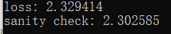
print('loss: %f' % loss)
print('sanity check: %f' % (-np.log(0.1)))
内联问题1:
为什么我们期望我们的损失接近-log(0.1)?
你的回答:因为我们没有执行学习过程,只是基于一些初始的随机权值计算softmax,我们预计初始损失必须接近-log(0.1),因为最初所有的类被选择的可能性是相等的。在CIFAR-10中,我们有10个类,因此正确类的概率是0.1,而softmax损耗是正确类的负对数概率,因此它是-log(0.1)。
In[21]:
使用数值梯度检查作为调试工具。
loss, grad = softmax_loss_naive(W, X_dev, y_dev, 0.0)
from cs231n.gradient_check import grad_check_sparse
f = lambda w: softmax_loss_naive(w, X_dev, y_dev, 0.0)[0]
grad_numerical = grad_check_sparse(f, W, grad, 10)

loss, grad = softmax_loss_naive(W, X_dev, y_dev, 5e1)
f = lambda w: softmax_loss_naive(w, X_dev, y_dev, 5e1)[0]
grad_numerical = grad_check_sparse(f, W, grad, 10)
numerical: 0.781850 analytic: 0.781850, relative error: 6.999032e-09
numerical: -2.422653 analytic: -2.422653, relative error: 8.423244e-09
numerical: -0.398160 analytic: -0.398161, relative error: 1.221467e-07
numerical: 2.088059 analytic: 2.088059, relative error: 2.205767e-08
numerical: 2.566471 analytic: 2.566471, relative error: 4.969465e-08
numerical: 1.499760 analytic: 1.499759, relative error: 2.717104e-08
numerical: 1.059147 analytic: 1.059147, relative error: 1.580263e-08
numerical: 0.985528 analytic: 0.985528, relative error: 1.346815e-08
numerical: -1.171883 analytic: -1.171883, relative error: 4.386754e-09
numerical: -3.564793 analytic: -3.564793, relative error: 1.531916e-08
numerical: 1.746211 analytic: 1.746211, relative error: 1.259174e-09
numerical: -1.018067 analytic: -1.018067, relative error: 6.152135e-09
numerical: 0.498837 analytic: 0.498837, relative error: 1.461814e-07
numerical: 1.725963 analytic: 1.725963, relative error: 3.551817e-08
numerical: 1.155462 analytic: 1.155462, relative error: 5.151725e-08
numerical: -4.052721 analytic: -4.052721, relative error: 2.070817e-08
numerical: -1.909706 analytic: -1.909706, relative error: 2.008640e-08
numerical: -1.998249 analytic: -1.998249, relative error: 1.588674e-09
numerical: -0.844575 analytic: -0.844575, relative error: 5.914254e-08
numerical: -2.580084 analytic: -2.580084, relative error: 8.707794e-09
完成softmax_loss_vectorized的填写
def softmax_loss_vectorized(W, X, y, reg):
    """
    Softmax loss function, vectorized version.

    Inputs and outputs are the same as softmax_loss_naive.
    """
    # Initialize the loss and gradient to zero.
    loss = 0.0
    dW = np.zeros_like(W)

    #############################################################################
    # TODO: Compute the softmax loss and its gradient using no explicit loops.  #
    # Store the loss in loss and the gradient in dW. If you are not careful     #
    # here, it is easy to run into numeric instability. Don't forget the        #
    # regularization!                                                           #
    #############################################################################
    # *****START OF YOUR CODE (DO NOT DELETE/MODIFY THIS LINE)*****

    N = X.shape[0]
    scores = X.dot(W)  # (N, C)
    scores1 = scores - np.max(scores, axis=1, keepdims=True)  # (N, C)
    loss1 = -scores1[range(N), y] + np.log(np.sum(np.exp(scores1), axis=1))  # (N,)
    loss = np.sum(loss1) / N + reg * np.sum(W ** 2)
    dloss1 = np.ones((N, 1)) / N  # (N, 1)
    dscores1 = dloss1 * np.exp(scores1) / np.sum(np.exp(scores1), axis=1, keepdims=True)  # (N, C)
    dscores1[[range(N)], y] -= dloss1.T
    dscores = dscores1  # (N, C)
    dW = X.T.dot(dscores) + 2 * reg * W

    # *****END OF YOUR CODE (DO NOT DELETE/MODIFY THIS LINE)*****

    return loss, dW
In[22]:
tic = time.time()
loss_naive, grad_naive = softmax_loss_naive(W, X_dev, y_dev, 0.000005)
toc = time.time()
print('naive loss: %e computed in %fs' % (loss_naive, toc - tic))

from cs231n.classifiers.softmax import softmax_loss_vectorized
tic = time.time()
loss_vectorized, grad_vectorized = softmax_loss_vectorized(W, X_dev, y_dev, 0.000005)
toc = time.time()
print('vectorized loss: %e computed in %fs' % (loss_vectorized, toc - tic))
#比较两个的差别
grad_difference = np.linalg.norm(grad_naive - grad_vectorized, ord='fro')
print('Loss difference: %f' % np.abs(loss_naive - loss_vectorized))
print('Gradient difference: %f' % grad_difference)
naive loss: 2.318560e+00 computed in 0.047872s
vectorized loss: 2.318560e+00 computed in 0.003992s
Loss difference: 0.000000
Gradient difference: 0.000000
采用交叉验证
ln[23]:
from cs231n.classifiers import Softmax
results = {}
best_val = -1
best_softmax = None
learning_rates = [1e-7, 2e-6, 2.5e-6]
regularization_strengths = [1e3, 1e4, 2e4, 2.5e4, 3e4, 3.5e4]

################################################################################
# TODO:                                                                        #
# Use the validation set to set the learning rate and regularization strength. #
# This should be identical to the validation that you did for the SVM; save    #
# the best trained softmax classifer in best_softmax.                          #
################################################################################
# Obtain all possible combinations
grid_search = [ (lr, rg) for lr in learning_rates for rg in regularization_strengths]

for lr, rg in grid_search:
    # Create a new Softmax instance
    softmax_model = Softmax()
    # Train the model with current parameters
    softmax_model.train(X_train, y_train, learning_rate=lr, reg=rg, num_iters=1000)
    # Predict values for training set
    y_train_pred = softmax_model.predict(X_train)
    # Calculate accuracy
    train_accuracy = np.mean(y_train_pred == y_train)
    # Predict values for validation set
    y_val_pred = softmax_model.predict(X_val)
    # Calculate accuracy
    val_accuracy = np.mean(y_val_pred == y_val)
    # Save results
    results[(lr,rg)] = (train_accuracy, val_accuracy)
    if best_val < val_accuracy:
        best_val = val_accuracy
        best_softmax = softmax_model

################################################################################
#                              END OF YOUR CODE                                #
################################################################################

for lr, reg in sorted(results):
    train_accuracy, val_accuracy = results[(lr, reg)]
    print('lr %e reg %e train accuracy: %f val accuracy: %f' % (
                lr, reg, train_accuracy, val_accuracy))

print('best validation accuracy achieved during cross-validation: %f' % best_val)
lr 1.000000e-07 reg 1.000000e+03 train accuracy: 0.241204 val accuracy: 0.248000
lr 1.000000e-07 reg 1.000000e+04 train accuracy: 0.329980 val accuracy: 0.347000
lr 1.000000e-07 reg 2.000000e+04 train accuracy: 0.330857 val accuracy: 0.342000
lr 1.000000e-07 reg 2.500000e+04 train accuracy: 0.328735 val accuracy: 0.341000
lr 1.000000e-07 reg 3.000000e+04 train accuracy: 0.319816 val accuracy: 0.332000
lr 1.000000e-07 reg 3.500000e+04 train accuracy: 0.317020 val accuracy: 0.330000
lr 2.000000e-06 reg 1.000000e+03 train accuracy: 0.392592 val accuracy: 0.391000
lr 2.000000e-06 reg 1.000000e+04 train accuracy: 0.345122 val accuracy: 0.350000
lr 2.000000e-06 reg 2.000000e+04 train accuracy: 0.305735 val accuracy: 0.314000
lr 2.000000e-06 reg 2.500000e+04 train accuracy: 0.309245 val accuracy: 0.317000
lr 2.000000e-06 reg 3.000000e+04 train accuracy: 0.297224 val accuracy: 0.303000
lr 2.000000e-06 reg 3.500000e+04 train accuracy: 0.306735 val accuracy: 0.325000
lr 2.500000e-06 reg 1.000000e+03 train accuracy: 0.393469 val accuracy: 0.386000
lr 2.500000e-06 reg 1.000000e+04 train accuracy: 0.313816 val accuracy: 0.330000
lr 2.500000e-06 reg 2.000000e+04 train accuracy: 0.299224 val accuracy: 0.296000
lr 2.500000e-06 reg 2.500000e+04 train accuracy: 0.287347 val accuracy: 0.295000
lr 2.500000e-06 reg 3.000000e+04 train accuracy: 0.276837 val accuracy: 0.293000
lr 2.500000e-06 reg 3.500000e+04 train accuracy: 0.293286 val accuracy: 0.293000
best validation accuracy achieved during cross-validation: 0.391000
在测试集进行验证
ln[24]:
y_test_pred = best_softmax.predict(X_test)
test_accuracy = np.mean(y_test == y_test_pred)
print('softmax on raw pixels final test set accuracy: %f' % (test_accuracy, ))
softmax on raw pixels final test set accuracy: 0.387000
内联问题-真或假
可以向训练集添加一个新的数据点,使SVM损失保持不变,但Softmax分类器损失不是这种情况。
你的答案:真
你的解释:假设我们添加一个新的数据点,导致分数(10、8、7),也支持向量机的优势是2和正确的类是1,那么这个数据的支持向量机损失将是0,因为它满足,也就是说,max(0,8 + 2 - 10)+max(0、7 + 2 - 10)= 0。因此,损失保持不变。但是对于Softmax分类器,损失就不会增加,即-log(Softmax (10)) = -log(0.84) = 0.17。这是因为SVM损失是局部客观的,也就是说,它不关心个人分数的细节,只需要满足边际。另一方面,Softmax分类器在计算损失时考虑所有的个体分数。
ln[25]:
可视化
w = best_softmax.W[:-1,:] # strip out the bias
w = w.reshape(32, 32, 3, 10)

w_min, w_max = np.min(w), np.max(w)

classes = ['plane', 'car', 'bird', 'cat', 'deer', 'dog', 'frog', 'horse', 'ship', 'truck']
for i in range(10):
    plt.subplot(2, 5, i + 1)

    # Rescale the weights to be between 0 and 255
    wimg = 255.0 * (w[:, :, :, i].squeeze() - w_min) / (w_max - w_min)
    plt.imshow(wimg.astype('uint8'))
    plt.axis('off')
    plt.title(classes[i])


 688
688


 被折叠的 条评论
为什么被折叠?
被折叠的 条评论
为什么被折叠?
 到【灌水乐园】发言


