


主要目的:
通过线性回归算法,根据已知的数据集进行训练得出一条较吻合的曲线。
相关概念:
回归曲线:可以直观呈现出数据集相关的关系,并可以进行预测。
梯度下降法:
cost function: 回归算法是一种监督学习算法,会有响应的数据与预测数据进行比对,损失函数就是一种预测数据与实际数据偏差的表征。
实验步骤:
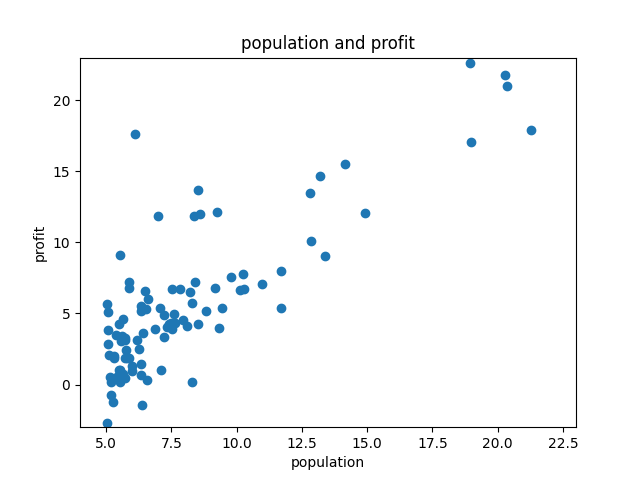
1:根据数据集画出对应的图
# Part two plotting
def plotData(x, y):
    plt.plot(x, y, 'rx', ms='10')
    plt.xlabel('Profit in $10,000s')
    plt.ylabel('Population of City in 10,000s')


print('plot data ....')
data = np.loadtxt('ex1data1.txt', delimiter=',')
X = data[:, 0]
Y = data[:, 1]
m = len(Y)
plotData(X, Y)
_ = input('Press [enter] to continue')
损失函数:
根据图片可以看出这是一个线性函数:我们可以先假设它为
h
(
x
)
=
θ
0
+
θ
1
x
h(x) = θ_0 + θ_1x
h(x)=θ0+θ1x
而现在我们需要做的就是得出这两个参数,即θ0 和 θ1,那么如何去做呢?我们可以随意的假设两个参数的值,并且画出它的曲线,看看是否与图像吻合,由于我们有图像作为标准,即,我们知道答案,所以这是一种有监督学习。现在当我们输入某一对参数时,对训练集进行训练,那么我们可以得出一个损失函数:
c
o
s
t
=
1
2
M
∑
(
h
θ
(
x
(
i
)
)
−
y
(
i
)
)
2
cost = \frac{1}{2M} \sum (h_\theta(x^{(i)}) - y^{(i)})^2
cost=2M1∑(hθ(x(i))−y(i))2
现在我们来构建损失函数:
实现:
def computeCost(x, y, theta):
    m = len(y)
    J = 0
    predictions = x.dot(theta)
    sqrErrors = (predictions - y) ** 2
    J = 1/(2*m) * np.sum(sqrErrors)
    return J
首先给X值一个额外参数,即截距
X = np.c_[np.ones(m), X] # add the extra parameter
测试损失函数:
先定义一个theta值,我们将它设为[0, 0],那么就有:
theta = np.zeros((2, ))
print('Testing the cost function')
J = computeCost(X, Y, theta)
print('With theta=[0, 0], Cost computed = %f' % J)
print('Expected cost value (approx) 32.07')
结果为:
Testing the cost function
With theta=[0, 0], Cost computed = 32.072734
Expected cost value (approx) 32.07
再更改theta值:
J = computeCost(X, Y, [-1, 2])
print('With theta=[-1, 2], Cost computed = %f' % J)
print('Expected cost value (approx) 54.24')
结果为:
With theta=[-1, 2], Cost computed = 54.242455
Expected cost value (approx) 54.24
可以明确的是cost越小那么曲线就吻合的更好,此时我们就需要使用梯度下降法来进行选择更吻合数据的 θ \theta θ
梯度下降:
定义:
θ
j
:
=
θ
j
−
α
∂
∂
θ
j
J
(
θ
0
,
θ
1
)
\theta_j := \theta_j - \alpha\frac{\partial}{\partial\theta_j}J(\theta_0,\theta_1)
θj:=θj−α∂θj∂J(θ0,θ1)
其中,
α
\alpha
α是学习率(learning rate),可以人为进行调控 := 这个符号代表的是赋值,,而且我们可以求出对应的
θ
\theta
θ偏导公式
θ
0
:
1
M
∑
(
h
θ
(
x
(
i
)
)
−
y
(
i
)
)
\theta_0 : \frac{1}{M} \sum(h_\theta(x^{(i)}) - y^{(i)})
θ0:M1∑(hθ(x(i))−y(i))
θ 1 : 1 M ∑ ( h θ ( x ( i ) ) − y ( i ) ) × x ( i ) \theta_1 : \frac{1}{M} \sum(h_\theta(x^{(i)}) - y^{(i)})\times x^{(i)} θ1:M1∑(hθ(x(i))−y(i))×x(i)
实现:
def gradientDescent(x, y, theta, alpha, num_iters):
    m = len(y)
    J_history = np.zeros((num_iters, ))
    for iter in range(num_iters):
        theta = theta - (alpha * (x.dot(theta) - y).dot(x)) / m
        J_history[iter] = computeCost(x, y, theta)
    return theta
确定循环参数:
iterations = 1500 # 循环次数
alpha = 0.01 # 学习率
循环更新theta:
print('Running Gradient Descent')
theta = gradientDescent(X, Y, theta, alpha, iterations)
print('theta found by gradient descent')
print(theta)
print('expected the value (approx) [-3.6303, 1.1664]')
结果为:
Running Gradient Descent
theta found by gradient descent
[-3.63029144  1.16636235]
expected the value (approx) [-3.6303, 1.1664]
绘制近似曲线:
plt.plot(X[:, 1], X.dot(theta), 'b-')
plt.legend(['Training data', 'Linear regression']) # 标签
plt.show()
结果为:

可见一次函数符合的还行,但是用其他的函数可能符合的会更佳,比如log, x \sqrt{x} x等等
预测:
经过上述步骤得到一个比较理想的值,接下来我们进行验证看看是否符合样本数据
# Predict values for population for size of 35000 and 70000
predict1 = np.dot([1, 3.5], theta)
print('For population = 35000, we predict a profit of ', predict1*10000)
predict2 = np.dot([1, 7], theta)
print('For population = 70000, we predict a profit of', predict2*10000)
_ = input('Press [enter] to continue')
结果为:
For population = 35000, we predict a profit of  4519.7678677017675
For population = 70000, we predict a profit of 45342.45012944712
梯度下降3d演示:
参数准备:
# Visualizing J(theta0, theta1)
print('Visualizing J(theta0, theta1)')

# Grid over which we will calculate J
theta0_vals = np.linspace(-10, 10, 100)
theta1_vlas = np.linspace(-1, 4, 100)

# initialize J_vlas to a matrix of 0's
J_vals = np.zeros((np.size(theta0_vals, ), np.size(theta1_vlas, )))

# Fill out J_vals
for i in range(np.size(theta0_vals, )):
    for j in range(np.size(theta1_vlas, )):
        t = np.array([theta0_vals[i], theta1_vlas[j]])
        J_vals[i][j] = computeCost(X, Y, t)
3d 绘制:
theta0_vals, theta1_vlas = np.meshgrid(theta0_vals, theta1_vlas)
fit = plt.figure()
ax = plt.axes(projection='3d')
ax.plot_surface(theta0_vals, theta1_vlas, J_vals)
ax.set_xlabel(r'$\theta$0')
ax.set_ylabel(r'$\theta$1')
如图:

等高线绘制:
fit2 = plt.figure()
ax2 = fit2.add_subplot(111)
ax2.contour(theta0_vals, theta1_vlas, J_vals, np.logspace(-1, 3, 20))
ax2.plot(theta[0], theta[1], 'rx', ms=10, lw=2)
ax2.set_xlabel(r'$\theta$0')
ax2.set_ylabel(r'$\theta$1')
plt.show()
如图:

完整代码请参考gitee地址:https://gitee.com/qingmoxuan/maching-learning.git
使用到的库:
import matplotlib.pyplot as plt
import numpy as np
总结:
使用到的库:
import matplotlib.pyplot as plt
import numpy as np
以上代码大体由matlab翻译从python,需要注意的是np关于数组的各种操作,以及2d,3d图的绘制。


 675
675


 被折叠的 条评论
为什么被折叠?
被折叠的 条评论
为什么被折叠?
 到【灌水乐园】发言


