学习笔记——sklearn监督学习：回归(简单数学知识罗列)

一、数学优化

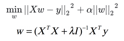
损失函数

损失函数（Loss function）是用来估量你模型的预测值与真实值的不一致程度，它是一个非负实值函数，通常用。损失函数越小，模型的鲁棒性就越好。损失函数是经验风险函数的核心部分，也是结构风险函数的重要组成部分。模型的风险结构包括了风险项和正则项，通常如下所示：

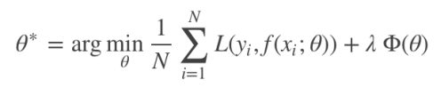
其中，前面的均值函数表示的是经验风险函数，L 代表的是损失函数，后面的 Φ是正则化项（regularizer）或者叫惩罚项（penalty term），它可以是 L1，也可以是L2，或者其他的正则函数。整个式子表示的意思是找到使目标函数最小时的θ值。

常见的损失误差有五种：

1. 0-1 损失（黑色）

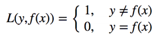
3. 铰链损失（Hinge Loss）：主要用于支持向量机（SVM） 中

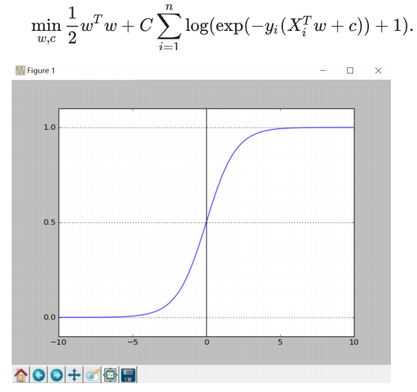
4. 互熵损失 （Cross Entropy Loss，Softmax Loss）：用于 Logistic 回归与 Softmax 分类中（红色）；

5. 平方损失（Square Loss）：主要是最小二乘法（OLS）中（略）；

6. 指数损失（Exponential Loss） ：主要用于 Adaboost 算法中（蓝色）；

---

SoftMax 损失

逻辑回归并没有求似然函数的极值，而是把极大化当做是一种思想，进而推导出它的经验风险函数为：最小化负的似然函数（即axF(y,f(x))→min−F(y,f(x)))maxF(y,f(x))→min−F(y,f(x))）。从损失函数的视角来看，它就成了 Softmax 损失函数了。

log 损失函数的标准形式：

利用已知的样本分布，找到最有可能（即最大概率）导致这种分布的参数值；或者说什么样的参数才能使我们观测到目前这组数据的概率最大。

---

二、回归分析

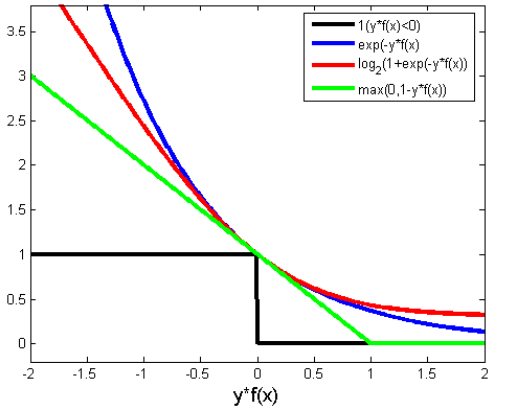
考虑广义线性模型：

其中 X 表示样本集，W 为待拟合的参数

1、最小二乘回归

2、岭回归

3、Logistics 回归

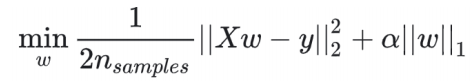
4、Lasso 回归

---

三、实例

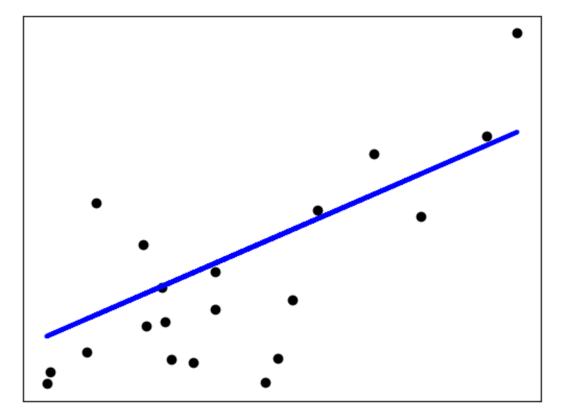
1、Linear Regression

import matplotlib.pyplot as plt
import numpy as np
from sklearn import datasets, linear_model
from sklearn.metrics import mean_squared_error, r2_score

# Load the diabetes dataset
diabetes = datasets.load_diabetes()


# Use only one feature
diabetes_X = diabetes.data[:, np.newaxis, 2]

# Split the data into training/testing sets
diabetes_X_train = diabetes_X[:-20]
diabetes_X_test = diabetes_X[-20:]

# Split the targets into training/testing sets
diabetes_y_train = diabetes.target[:-20]
diabetes_y_test = diabetes.target[-20:]

# Create linear regression object
regr = linear_model.LinearRegression()

# Train the model using the training sets
regr.fit(diabetes_X_train, diabetes_y_train)

# Make predictions using the testing set
diabetes_y_pred = regr.predict(diabetes_X_test)

# The coefficients
print('Coefficients: \n', regr.coef_)
# The mean squared error
print("Mean squared error: %.2f"
      % mean_squared_error(diabetes_y_test, diabetes_y_pred))
# Explained variance score: 1 is perfect prediction
print('Variance score: %.2f' % r2_score(diabetes_y_test, diabetes_y_pred))

# Plot outputs
plt.scatter(diabetes_X_test, diabetes_y_test,  color='black')
plt.plot(diabetes_X_test, diabetes_y_pred, color='blue', linewidth=3)

plt.xticks(())
plt.yticks(())

plt.show()

结果：

('Coefficients: \n', array([938.23786125]))
Mean squared error: 2548.07
Variance score: 0.47

---

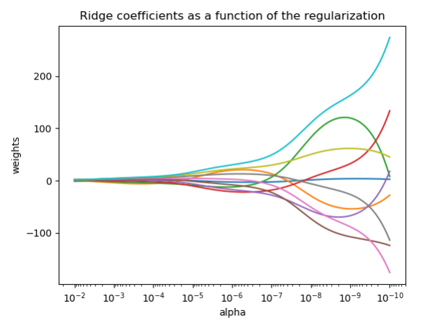
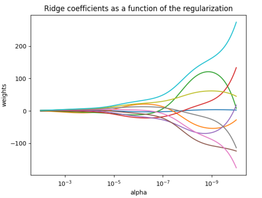
2、Ridge Regression

import numpy as np
import matplotlib.pyplot as plt
from sklearn import linear_model

# X is the 10x10 Hilbert matrix
X = 1. / (np.arange(1, 11) + np.arange(0, 10)[:, np.newaxis])
y = np.ones(10)

# #####################################################################
# Compute paths

n_alphas = 200
alphas = np.logspace(-10, -2, n_alphas)

coefs = []
for a in alphas:
    ridge = linear_model.Ridge(alpha=a, fit_intercept=False)
    ridge.fit(X, y)
    coefs.append(ridge.coef_)

# ####################################################################
# Display results

ax = plt.gca()

ax.plot(alphas, coefs)
ax.set_xscale('log')
ax.set_xlim(ax.get_xlim()[::-1])  # reverse axis
plt.xlabel('alpha')
plt.ylabel('weights')
plt.title('Ridge coefficients as a function of the regularization')
plt.axis('tight')
plt.show()

结果：

---

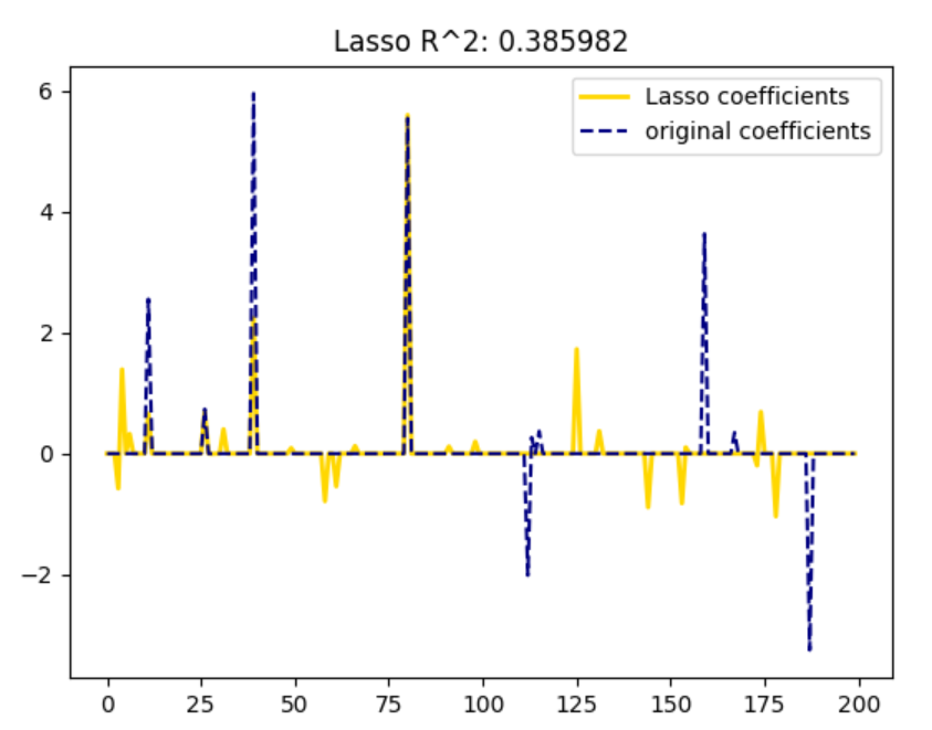
3、Lasso

import numpy as np
import matplotlib.pyplot as plt

from sklearn.metrics import r2_score

# #############################################################################
# Generate some sparse data to play with
np.random.seed(42)

n_samples, n_features = 50, 200
X = np.random.randn(n_samples, n_features)
coef = 3 * np.random.randn(n_features)
inds = np.arange(n_features)
np.random.shuffle(inds)
coef[inds[10:]] = 0  # sparsify coef
y = np.dot(X, coef)

# add noise
y += 0.01 * np.random.normal(size=n_samples)

# Split data in train set and test set
n_samples = X.shape[0]
X_train, y_train = X[:n_samples // 2], y[:n_samples // 2]
X_test, y_test = X[n_samples // 2:], y[n_samples // 2:]

# #############################################################################
# Lasso
from sklearn.linear_model import Lasso

alpha = 0.1
lasso = Lasso(alpha=alpha)

y_pred_lasso = lasso.fit(X_train, y_train).predict(X_test)
r2_score_lasso = r2_score(y_test, y_pred_lasso)
print(lasso)
print("r^2 on test data : %f" % r2_score_lasso)

plt.plot(lasso.coef_, color='gold', linewidth=2,
         label='Lasso coefficients')
plt.plot(coef, '--', color='navy', label='original coefficients')
plt.legend(loc='best')
plt.title("Lasso R^2: %f"
          % (r2_score_lasso))
plt.show()

结果：

Lasso(alpha=0.1)
r^2 on test data : 0.385982

---

4、Logistics Regression

import numpy as np
import matplotlib.pyplot as plt
from sklearn.linear_model import LogisticRegression
from sklearn import datasets

# import some data to play with
iris = datasets.load_iris()
X = iris.data[:, :2]  # we only take the first two features.
Y = iris.target

logreg = LogisticRegression(C=1e5, solver='lbfgs', multi_class='multinomial')

# Create an instance of Logistic Regression Classifier and fit the data.
logreg.fit(X, Y)

# Plot the decision boundary. For that, we will assign a color to each
# point in the mesh [x_min, x_max]x[y_min, y_max].
x_min, x_max = X[:, 0].min() - .5, X[:, 0].max() + .5
y_min, y_max = X[:, 1].min() - .5, X[:, 1].max() + .5
h = .02  # step size in the mesh
xx, yy = np.meshgrid(np.arange(x_min, x_max, h), np.arange(y_min, y_max, h))
Z = logreg.predict(np.c_[xx.ravel(), yy.ravel()])

# Put the result into a color plot
Z = Z.reshape(xx.shape)
plt.figure(1, figsize=(4, 3))
plt.pcolormesh(xx, yy, Z, cmap=plt.cm.Paired)

# Plot also the training points
plt.scatter(X[:, 0], X[:, 1], c=Y, edgecolors='k', cmap=plt.cm.Paired)
plt.xlabel('Sepal length')
plt.ylabel('Sepal width')

plt.xlim(xx.min(), xx.max())
plt.ylim(yy.min(), yy.max())
plt.xticks(())
plt.yticks(())

plt.show()

结果：