【笔记】【机器学习基础】分类器的不确定估计

分类器除了给出预测的不确定度，还能给出对这个预测的置信程度。
函数：1、decision_function 2、predict_proba
下面通过构建GradientBoostingClassifier分类测试：

from sklearn.ensemble import GradientBoostingClassifier
from sklearn.datasets import make_circles
X, y = make_circles(noise=0.25, factor=0.5, random_state=1)

y_named = np.array(["blue", "red"])[y]

X_train, X_test, y_train_named, y_test_named, y_train, y_test = \
    train_test_split(X, y_named, y, random_state=0)

gbrt = GradientBoostingClassifier(random_state=0)
gbrt.fit(X_train, y_train_named)

一、决策函数

（1）返回值

print("X_test.shape:", X_test.shape)
print("Decision function shape:",
      gbrt.decision_function(X_test).shape)

X_test.shape: (25, 2)
Decision function shape: (25,)
对于类别1，这个值表示该数据点属于正类的置信程度
正值表示对正类的偏好，负值表示对其他类的偏好

（2）显示decision_function前几个元素

print("Decision function:", gbrt.decision_function(X_test)[:6])

（3）查看决策函数的正负号再现预测值

print("Thresholded decision function:\n",
      gbrt.decision_function(X_test) > 0)
print("Predictions:\n", gbrt.predict(X_test))

Thresholded decision function:
[ True False False False True True False True True True False True
True False True False False False True True True True True False
False]
Predictions:
[‘red’ ‘blue’ ‘blue’ ‘blue’ ‘red’ ‘red’ ‘blue’ ‘red’ ‘red’ ‘red’ ‘blue’
‘red’ ‘red’ ‘blue’ ‘red’ ‘blue’ ‘blue’ ‘blue’ ‘red’ ‘red’ ‘red’ ‘red’
‘red’ ‘blue’ ‘blue’]
对于二分类问题，反类是classes_属性的第一个元素，正类是第二个元素。完全在现predict的输出需要利用classes_属性：
（4）再现predict的输出

greater_zero = (gbrt.decision_function(X_test) > 0).astype(int)

pred = gbrt.classes_[greater_zero]

print("pred is equal to predictions:",
      np.all(pred == gbrt.predict(X_test)))

pred is equal to predictions: True

（5）

decision_function = gbrt.decision_function(X_test)
print("Decision function minimum: {:.2f} maximum: {:.2f}".format(
      np.min(decision_function), np.max(decision_function)))

decision_function任意范围取值，取决于数据和模型参数，所以输出往往会很难解释

（6）利用颜色编码在二维平面将所有点的decision_function和决策边界可视化

fig, axes = plt.subplots(1, 2, figsize=(13, 5))
mglearn.tools.plot_2d_separator(gbrt, X, ax=axes[0], alpha=.4,
                                fill=True, cm=mglearn.cm2)
scores_image = mglearn.tools.plot_2d_scores(gbrt, X, ax=axes[1],
                                            alpha=.4, cm=mglearn.ReBl)

for ax in axes:
    # plot training and test points
    mglearn.discrete_scatter(X_test[:, 0], X_test[:, 1], y_test,
                             markers='^', ax=ax)
    mglearn.discrete_scatter(X_train[:, 0], X_train[:, 1], y_train,
                             markers='o', ax=ax)
    ax.set_xlabel("Feature 0")
    ax.set_ylabel("Feature 1")
cbar = plt.colorbar(scores_image, ax=axes.tolist())
cbar.set_alpha(1)
cbar.draw_all()
axes[0].legend(["Test class 0", "Test class 1", "Train class 0",
                "Train class 1"], ncol=4, loc=(.1, 1.1))

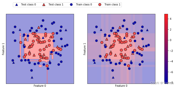
给出预测结果和分类器的置信程度。但是上面的图像难以分辨决策边界

二、预测概率

（1）predict_proba

print("Shape of probabilities:", gbrt.predict_proba(X_test).shape)

predict_proba的输出是每个类别的概率

（2）估计概率

print("Predicted probabilities:")
print(gbrt.predict_proba(X_test[:6]))

Predicted probabilities:
[[0.016 0.984]
[0.846 0.154]
[0.981 0.019]
[0.974 0.026]
[0.014 0.986]
[0.025 0.975]]
每行的第一个元素是第一个类别的估计概率，第二个元素是第二个类别的估计概率，两个类别的元素之和始终为1

（3）梯度提升模型的决策边界和预测概率

fig, axes = plt.subplots(1, 2, figsize=(13, 5))
    
mglearn.tools.plot_2d_separator(
    gbrt, X, ax=axes[0], alpha=.4, fill=True, cm=mglearn.cm2)
scores_image = mglearn.tools.plot_2d_scores(
    gbrt, X, ax=axes[1], alpha=.5, cm=mglearn.ReBl, function='predict_proba')

for ax in axes:
    # plot training and test points
    mglearn.discrete_scatter(X_test[:, 0], X_test[:, 1], y_test,
                             markers='^', ax=ax)
    mglearn.discrete_scatter(X_train[:, 0], X_train[:, 1], y_train,
                             markers='o', ax=ax)
    ax.set_xlabel("Feature 0")
    ax.set_ylabel("Feature 1")

cbar = plt.colorbar(scores_image, ax=axes.tolist())
cbar.set_alpha(1)
cbar.draw_all()
axes[0].legend(["Test class 0", "Test class 1", "Train class 0",
                "Train class 1"], ncol=4, loc=(.1, 1.1))

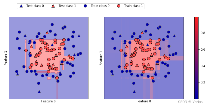
边界更明显

三、多分类问题的不确定度

将两个函数应用于多分类问题

（1）鸢尾花数据集

from sklearn.datasets import load_iris

iris = load_iris()
X_train, X_test, y_train, y_test = train_test_split(
    iris.data, iris.target, random_state=42)

gbrt = GradientBoostingClassifier(learning_rate=0.01, random_state=0)
gbrt.fit(X_train, y_train)

print("Decision function shape:", gbrt.decision_function(X_test).shape)

print("Decision function:")
print(gbrt.decision_function(X_test)[:6, :])

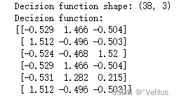
对于多分类的，decision_function 的形状为（n_samples，n_classes)，每一类对应每个类别的确定度分数，分数较高的类别可能性更大。

（2）再现预测结果

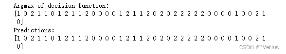
print("Argmax of decision function:")
print(np.argmax(gbrt.decision_function(X_test), axis=1))
print("Predictions:")
print(gbrt.predict(X_test))

（3）

print("Predicted probabilities:")
print(gbrt.predict_proba(X_test)[:6])

print("Sums:", gbrt.predict_proba(X_test)[:6].sum(axis=1))

Predicted probabilities:
[[0.107 0.784 0.109]
[0.789 0.106 0.105]
[0.102 0.108 0.789]
[0.107 0.784 0.109]
[0.108 0.663 0.228]
[0.789 0.106 0.105]]
Sums: [1. 1. 1. 1. 1. 1.]

（4）再现预测结果（通过predict_proba的argmax）

print("Argmax of predicted probabilities:")
print(np.argmax(gbrt.predict_proba(X_test), axis=1))
print("Predictions:")
print(gbrt.predict(X_test))

predict_proba和decision_function的形状始终相同，除了二分类下的decision_function

（5）通过classes_获取真实属性名称

logreg = LogisticRegression()
named_target = iris.target_names[y_train]
logreg.fit(X_train, named_target)
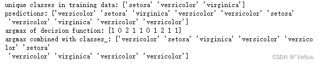
print("unique classes in training data:", logreg.classes_)
print("predictions:", logreg.predict(X_test)[:10])
argmax_dec_func = np.argmax(logreg.decision_function(X_test), axis=1)
print("argmax of decision function:", argmax_dec_func[:10])
print("argmax combined with classes_:",
      logreg.classes_[argmax_dec_func][:10])