


二,分类——感知机
5.3.1确定训练数据
(我们可以发现y值有+1,-1的区别,我们选择用原点表示y=1的数据,用叉号表示y=-1的数据
重要代码如图: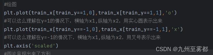
引入训练数据运行结果如下:
5,3,2感知机的实现

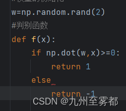
由于参数为w所以进行w的初始化。并进行判别式的定义。
更新w的值进行不断训练 ,公式如下:

假设重复次数是10次,不断更新w的值,运用for循环
for _ in range(epoch):输出日志来展示

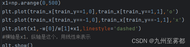
画一条直线来使权重向量变为法线向量
图形如图所示:

可以看到效果比较好。
5.3.3验证
对于建立的模型我们输入两组图像的像素来判断
 结果如图
结果如图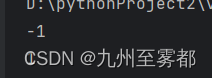
感知机程序如下:
import numpy as np
import matplotlib.pyplot as plt
#读入训练数据
train =np.loadtxt('images1.csv',delimiter=',',skiprows=1)
#引入训练数据的语句
train_x=train[:,0:2]
train_y=train[:,2]

#绘图
#plt.plot(train_x[train_y==1,0],train_x[train_y==1,1],'o')
#可以这么理解在y=1的情况下,横轴为x1,纵轴为x2,用实心圆表示出来
#plt.plot(train_x[train_y==-1,0],train_x[train_y==-1,1],'x')
#可以这么理解在y=-1的情况下,横轴为x1,纵轴为x2,用叉号表示出来
#plt.axis('scaled')
#图片呈现出来了方形
#plt.show()
#权重的初始化
w=np.random.rand(2)
#判别函数
def f(x):
    if np.dot(w,x)>=0:
        return 1
    else:
        return -1
#重复次数
epoch=10
#更新次数
count=0
#学习权重
for _ in range(epoch):
  for x,y in zip(train_x,train_y):#x,y在序列里面
      if f(x)!=y:
        w = w + y *x#更新
        #输出日志
        count=count+1
       # print('第{}次:w={}'.format(count,w))
#画一条直线,使权重向量成为法线向量的直线方程是内积为0的x的集合,
#w*x=w1*x1+w2*x2=0
x2=-w1/w2*x1
x1=np.arange(0,500)
plt.plot(train_x[train_y==1,0],train_x[train_y==1,1],'o')
plt.plot(train_x[train_y==-1,0],train_x[train_y==-1,1],'x')
plt.plot(x1,-w[0]/w[1]*x1,linestyle='dashed')
#横轴是x1,纵轴是这个,用线性来表示
plt.show()
#print(f([100,300]))
#纵向是-1
#print(f([400,120]))
#横向是1
5.4分类-逻辑回归
5.4.1确定训练数据
在逻辑回归中,我们需要把横向分配为1.纵向分配为0
5.4.2逻辑回归的实现
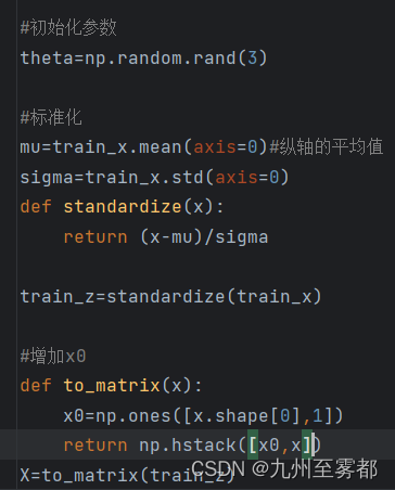
1.初始化参数
2.训练数据标准化,x1,x2分别标准化,不要忘了加x0列
标准化代码如图:
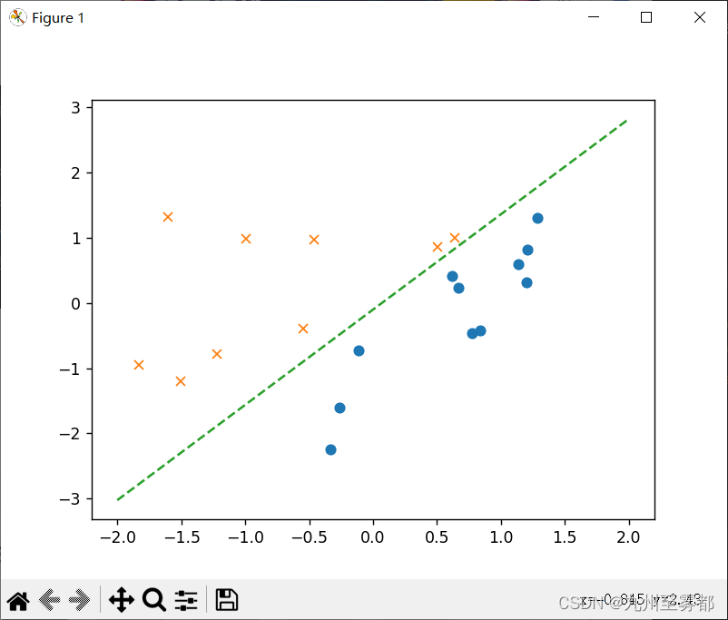
绘图结果如图:

3.预测函数-sigmod函数


准备工作完成。
接下来准备逐步更新参数:

由于theta转置乘以x=0这是决策边界
其>=0时是横向的
其<0是纵向

画一下决策边界。

代码运行结果如图:
4.验证
1.直接输出结果:![]()
![]()
选择用整型数字输出:定义classify()


最终代码如下:
import numpy as np
import matplotlib.pyplot as plt

#读入训练数据
train=np.loadtxt('images2.csv',delimiter=',',skiprows=1)
#引入训练数据的语句
train_x=train[:,0:2]
train_y=train[:,2]

#初始化参数
theta=np.random.rand(3)

#标准化
mu=train_x.mean(axis=0)#纵轴的平均值
sigma=train_x.std(axis=0)
def standardize(x):
    return (x-mu)/sigma

train_z=standardize(train_x)

#增加x0
def to_matrix(x):
    x0=np.ones([x.shape[0],1])
    return np.hstack([x0,x])
X=to_matrix(train_z)

#sigmod函数
def f(x):
    return 1/(1+np.exp(-np.dot(x,theta)))#指数函数

#分类函数
def classify(x):
    return (f(x)>=0.5).astype(int)
#标准化
#更新参数
#学习率定义
ETA=1e-3
#重复次数为5000
epoch=5000
#更新次数
count=0

#重复学习
for _ in range(epoch):
    theta=theta-ETA*np.dot(f(X) - train_y,X)
    #日志输出
    count+=1
    print('第{}次:theta={}'.format(count,theta))


#classify(to_matrix(standardize([[200,100],[100,200]])))
#print(classify(to_matrix(standardize([[200,100],[100,200]]))))

#将训练数据画成图
x0=np.linspace(-2,2,100)#横轴
plt.plot(train_z[train_y==1,0],train_z[train_y==1,1],'o')
plt.plot(train_z[train_y==0,0],train_z[train_y==0,1],'x')
plt.plot(x0,-(theta[0]+theta[1]*x0)/theta[2],linestyle='dashed')
#用代码表现出公式,横轴是x,纵轴是公式
plt.show()
5.4.4线性不可分分类的实现
1.建立数据data3.csv
2.将数据绘图出来

看起来无法用直线来进行分类,所以我们选择用二次函数来分类
在训练数据中增加x2,即在theta中增加theta3,这样总参数就是四个
如上面所述,进行重复学习
绘图来表示结果:(对于有四个参数的式子,绘图公式如下)、

代码如下:
import numpy as np
import matplotlib.pyplot as plt
#读入训练数据
train=np.loadtxt('data3.csv',delimiter=',',skiprows=1)
#引入训练数据的语句
train_x=train[:,0:2]
train_y=train[:,2]

#参数初始化
theta=np.random.rand(4)#theta参数为4个
#标准化
mu=train_x.mean(axis=0)
sigma=train_x.std(axis=0)
def standardize(x):
    return (x-mu)/sigma
train_z=standardize(train_x)

#增加x0和x3
def to_matrix(x):
    x0=np.ones([x.shape[0],1])
    x3=x[:,0,np.newaxis]**2
    return np.hstack([x0,x,x3])
X=to_matrix(train_z)

#sigmod函数
def f(x):
    return 1/(1+np.exp(-np.dot(x,theta)))
#学习部分
#学习率
ETA=1e-3
#重复次数
epoch=5000
#重复学习
for _ in range(epoch):
    theta=theta-ETA*np.dot(f(X)-train_y,X)


#将训练数据画成图
#绘图
x1=np.linspace(-2,2,100)
x2= -(theta[0]+theta[1]*x1+theta[3]*x1**2)/theta[2]


#x0=np.linspace(-2,2,100)#横轴
plt.plot(train_z[train_y==1,0],train_z[train_y==1,1],'o')
plt.plot(train_z[train_y==0,0],train_z[train_y==0,1],'x')
#plt.plot(x0,-(theta[0]+theta[1]*x0)/theta[2],linestyle='dashed')
#用代码表现出公式,横轴是x,纵轴是公式
plt.plot(x1,x2,linestyle='dashed')
plt.show()
运行结果:
此时决策边界已经变成曲线。
我们和回归时一样,把重复次数作为横轴,精度作为纵轴来绘图 ,这可以看到精度上升的样子
计算表达式如图:

这个数值表示被正确分类的数据个数占总个数的比重
我们绘图来验证。
代码如下:
import numpy as np
import matplotlib.pyplot as plt
#读入训练数据
train=np.loadtxt('data3.csv',delimiter=',',skiprows=1)
#引入训练数据的语句
train_x=train[:,0:2]
train_y=train[:,2]

#参数初始化
theta=np.random.rand(4)#theta参数为4个
#标准化
mu=train_x.mean(axis=0)
sigma=train_x.std(axis=0)
def standardize(x):
    return (x-mu)/sigma
train_z=standardize(train_x)

#增加x0和x3
def to_matrix(x):
    x0=np.ones([x.shape[0],1])
    x3=x[:,0,np.newaxis]**2
    return np.hstack([x0,x,x3])
X=to_matrix(train_z)

#sigmod函数
def f(x):
    return 1/(1+np.exp(-np.dot(x,theta)))
#精度函数
def classify(x):
    return (f(x)>=0.5).astype(int)
#学习部分
#学习率
ETA=1e-3
#重复次数
epoch=5000
#精度的历史记录
accuracies = []
#重复学习
for _ in range(epoch):
    theta=theta-ETA*np.dot(f(X)-train_y,X)
    #计算现在的精度
    result=classify(X)==train_y
    accuracy=len(result[result==True])/len(result)
    accuracies.append(accuracy)


#将精度画成图
x=np.arange(len(accuracies))
plt.plot(x,accuracies)
plt.show()
图像如下:
5.4.5 随机梯度下降法的实现
把学习部分稍微改变一下:

完整代码如下:
import numpy as np
import matplotlib.pyplot as plt
#读入训练数据
train=np.loadtxt('data3.csv',delimiter=',',skiprows=1)
#引入训练数据的语句
train_x=train[:,0:2]
train_y=train[:,2]

#参数初始化
theta=np.random.rand(4)#theta参数为4个
#标准化
mu=train_x.mean(axis=0)
sigma=train_x.std(axis=0)
def standardize(x):
    return (x-mu)/sigma
train_z=standardize(train_x)

#增加x0和x3
def to_matrix(x):
    x0=np.ones([x.shape[0],1])
    x3=x[:,0,np.newaxis]**2
    return np.hstack([x0,x,x3])
X=to_matrix(train_z)

#sigmod函数
def f(x):
    return 1/(1+np.exp(-np.dot(x,theta)))
#学习部分
#学习率
ETA=1e-3
#重复次数
epoch=5000
#重复学习
for _ in range(epoch):
    #使用随机梯度下降法更新参数
    p=np.random.permutation(X.shape[0])
    for x,y in zip(X[p,:],train_y[p]):
        theta=theta-ETA*(f(x)-y)*x


#将训练数据画成图
#绘图
x1=np.linspace(-2,2,100)
x2= -(theta[0]+theta[1]*x1+theta[3]*x1**2)/theta[2]


#x0=np.linspace(-2,2,100)#横轴
plt.plot(train_z[train_y==1,0],train_z[train_y==1,1],'o')
plt.plot(train_z[train_y==0,0],train_z[train_y==0,1],'x')
#plt.plot(x0,-(theta[0]+theta[1]*x0)/theta[2],linestyle='dashed')
#用代码表现出公式,横轴是x,纵轴是公式
plt.plot(x1,x2,linestyle='dashed')
plt.show()
运行结果如图:

分类效果很不错。


 189
189


 被折叠的 条评论
为什么被折叠?
被折叠的 条评论
为什么被折叠?
 到【灌水乐园】发言


