Python绘图--函数图像（并计算三个函数相交围成的图像面积）

题目给出三个已知函数方程：

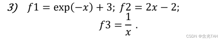
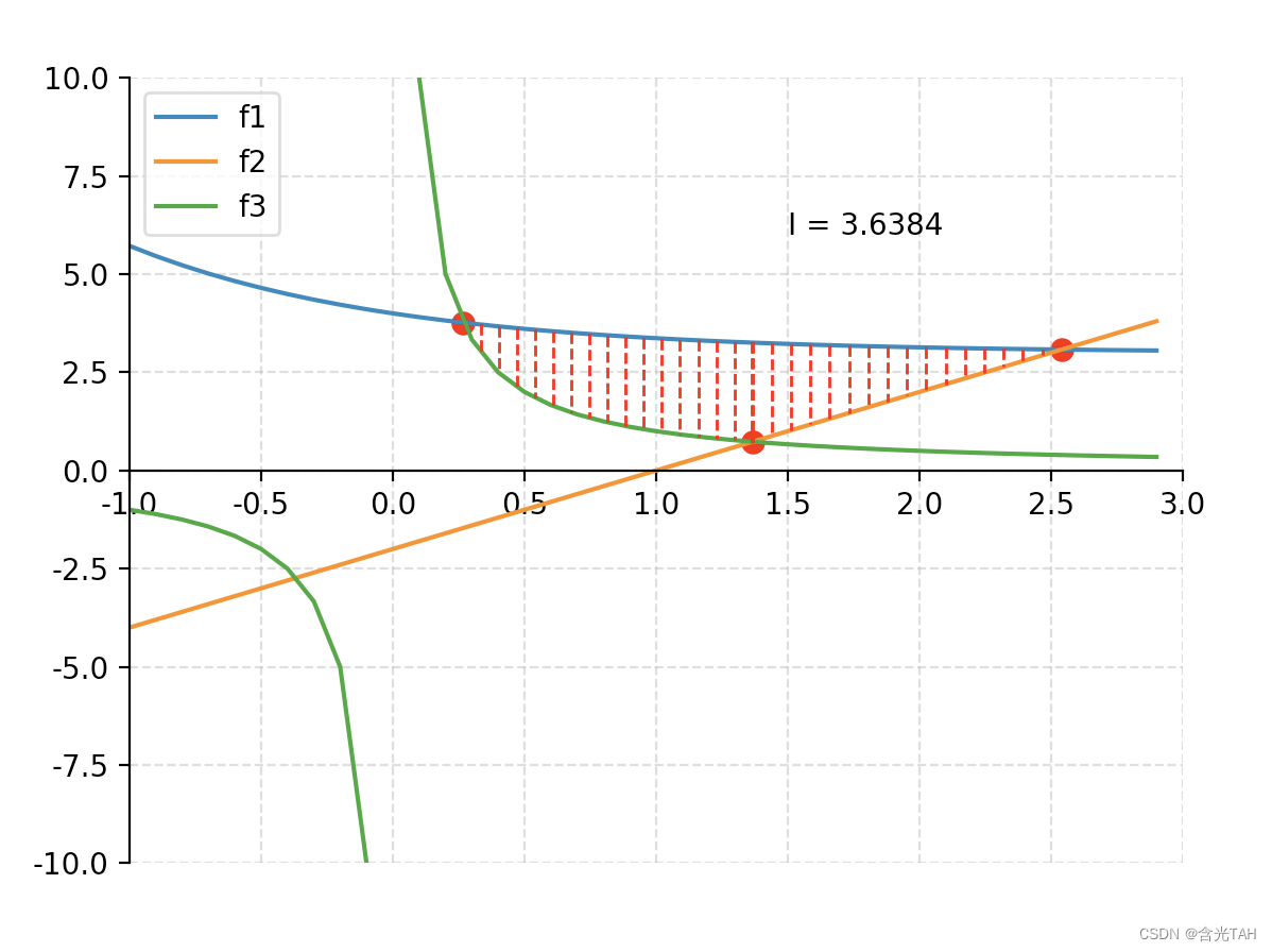
需要，首先画出函数图像，并且给所围图形打上阴影，并用计算其积分，运行效果如下：

具体代码：

import numpy as np # 给numpy库起个别名
from matplotlib import pyplot as plt  #matplotlib是Python语言及其数值计算库NumPy的绘图库。

#设置图像细节
#plt.rcParams['font.sans-serif'] = ['SimHei']  # 用来正常显示中文标签
plt.rcParams['axes.unicode_minus'] = False  # 用来正常显示负号
#plt.legend(loc= 'lower left') # 设置图例位置location
plt.ylim(-10, 10)  # y轴显示区间
plt.xlim(-1, 3)  # x轴显示区间


ax = plt.gca() #可以使用 plt.gcf()和 plt.gca()获得当前的图表和坐标轴(分别表示 Get Current Figure 和 Get Current Axes)
ax.xaxis.set_ticks_position('bottom') #设置x轴为下边框
ax.spines['bottom'].set_position(('data', 0))  # spines是脊柱的意思，移动x轴
ax.spines['top'].set_color('none')  # 设置顶部支柱的颜色为空
ax.spines['right'].set_color('none')  # 设置右边支柱的颜色为空
plt.grid(True, linestyle='--', alpha=0.5)  # 网格

X1 = np.arange(-1, 3, 0.1)  # x范围
X2 = np.ma.masked_array(X1, mask=((X1 < 0.000001) & (X1 > -0.000001)))  # 反比例函数去掉X为零的情况

F1 = np.exp(-X1) + 3  # 指数函数
F2 = 2 * X1 - 2  # 一次函数
F3 = 1 / X2  # 反比例函数


def f1(x):  # 指数函数
    return np.exp(-x) + 3


def f2(x):  # 一次函数
    return 2 * float(x) - 2 # 强制类型转换float


def f3(x):  # 反比例函数
    return 1 / float(x)



def root(f, g, a, b, eps1):
    while b - a > eps1:
        # 二分法 求f = g 方程的根
        x = (a + b) / 2
        y = f(x) - g(x)
        ya = f(a) - g(a)
        yb = f(b) - g(b)
        if y * ya < 0:
            b = x
        elif y * yb < 0:
            a = x
    r = "%.4f" % ((a + b) / 2)
    return r


def integral(f, a, b, eps2):
    # 设置初始积分
    n = 20
    # n对应的积分值
    R = [] # 一个空的list
    I = 0
    h = (b - a) / n
    # 计算积分
    for i in range(0, n - 1):
        I += (f(a + (i + 0.5) * h))
    R.append(h * I) # 记录h*I 的值
    while (1):
        # 更新
        n *= 2
        I = 0
        h = (b - a) / n
        # 计算
        for i in range(0, n - 1): # 从0 ～n-1的循环
            I += (f(a + (i + 0.5) * h)) # 矩形公式
        R.append(h * I)
        # 判断
        if (abs(R[-1] - R[-2]) / 3 < eps2):
            break
    c = []  # 存下每个积分点的横坐标
    for i in range(0, n - 1):
        c.append(a + h * i)
    # print("R:", R[-1])
    return c, R[-1]


def drawRomberg(f1, f2, a, b, eps2, n): #画出求积部分
    x1, y1 = integral(f1, a, b, eps2)
    x1_ = []
    for i in range(len(x1)):
        if i % n == 0:
            x1_.append(x1[i])
        if i == len(x1) - 1:
            x1_.append(x1[i])
    for i in x1_:
        line = [i, f1(i), i, f2(i)]
        plt.plot(line[::2], line[1::2], color='red',
                 linewidth=1, linestyle="--")


if __name__ == '__main__': #“if __name__==’__main__:”也像是一个标志，象征着Java等语言中的程序主入口，告诉其他程序员，代码入口在此——这是“if __name__==’__main__:”这条代码的意义之一。
    # 计算四个交点的坐标
    x4 = "%.4f" % float(root(f1, f2, 2, 3, 0.001))
    y4 = "%.4f" % float(f2(x4))
    x2 = "%.4f" % float(root(f1, f3, 0.1, 1, 0.001))
    y2 = "%.4f" % float(f3(x2))
    x3 = "%.4f" % float(root(f2, f3, 1, 2, 0.001))
    y3 = "%.4f" % float(f2(x3))
    x1 = "%.4f" % float(root(f2, f3, -1, -0.1, 0.001))
    y1 = "%.4f" % float(f2(x1))
    print("x1:%.4f" % float(x1), "y1:%.4f" % float(y1))
    print("x2:%.4f" % float(x2), "y2:%.4f" % float(y2))
    print("x3:%.4f" % float(x3), "y3:%.4f" % float(y3))
    print("x4:%.4f" % float(x4), "y4:%.4f" % float(y4))

    # 画出初始的三条函数
    plt.plot(X1, F1, linewidth=1.5, linestyle="-", label="f1")
    plt.plot(X1, F2, linewidth=1.5, linestyle="-", label="f2")
    plt.plot(X2, F3, linewidth=1.5, linestyle="-", label="f3")

    # 画出四个交点围成的三角形
    polygon = [[float(x2), float(y2)], [float(x3), float(y3)], [
        float(x4), float(y4)]]
    # line_area = polygon+[polygon[0]]
    # plt.plot([i[0] for i in line_area], [i[1] for i in line_area])

    # 画出三个焦点
    plt.scatter(polygon[0][0], polygon[0][1], s=50, c='r')
    plt.scatter(polygon[1][0], polygon[1][1], s=50, c='r')
    plt.scatter(polygon[2][0], polygon[2][1], s=50, c='r')

    # 计算面积
    I = integral(f1, float(x2), float(x4), 0.001)[1] - integral(f2, float(x3),
                                                                float(x4), 0.001)[1] - \
        integral(f3, float(x2), float(x3), 0.001)[1]

    # 画出求积部分
    drawRomberg(f1, f3, float(x2), float(x3), 0.001, 80)
    drawRomberg(f1, f2, float(x3), float(x4), 0.001, 80)

    # 显示计算结果
    plt.text(1.5, 6, "I = {}".format("%.4f" % float(I)))

    # 显示
    plt.legend(loc='upper left')
    plt.show()