


1、TensorFlow处理结构
TensorFlow基于数据流用于大规模分布式数值计算的开源框架。节点表示某种抽象的计算,边表示节点之间相互联系的张量。其计算流程为: 首先定义神经网络结构(数据流图 data flow graphs),再把数据 (数据以张量tensor形式存在) 放入结构中进行运算和训练。即tensor不断在一个节点flow到另一个节点。
- 建立结构
- 把数据放在结构里面
- 向量流动,参数进一步完善提升,作为下一次的数据,经过很多次的循环处理,令参数达到要求。

.
# 以计算函数y = 0.1x + 0.3的系数为例
import tensorflow as tf
import numpy as np
tf.compat.v1.disable_eager_execution()
#create data,创建数据集
x_data = np.random.rand(100).astype(np.float32) # 传入计算的值x
y_data = x_data * 0.1 + 0.3 # 真实值,权重系数=0.1,偏置系数=0.3
###create tensorflow structure start ###
# 用一个随机数列生成 1 列,-1到1的范围
Weights = tf.Variable(tf.random.uniform([1],-1.0,1.0))
# 将初始值为 0,一步步学习到0.1及0.3
biases = tf.Variable(tf.zeros([1]))
y = Weights * x_data + biases
# 预测的y与真实值的差别,最小化方差
# tf.reduce_mean 函数用于计算张量tensor沿着指定的数轴(tensor的某一维度)上的的平均值,主要用作降维或者计算tensor(图像)的平均值。
loss = tf.reduce_mean(tf.square(y - y_data))
# 选择优化器,0.6为学习效率.
train = tf.compat.v1.train.GradientDescentOptimizer(0.6).minimize(loss)
# 前面只是建立结构,需要初始化变量
init = tf.compat.v1.global_variables_initializer()
###create tensorflow structure end ###
#结构激活
sess = tf.compat.v1.Session()
#这里激活,sess是一个指针
sess.run(init) #very important
for step in range(201):
#开始训练
sess.run(train)
# 每隔20次输出结果
if step % 20 == 0:
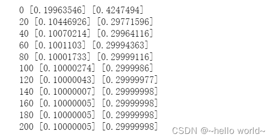
print(step,sess.run(Weights),sess.run(biases))
运算结果:
.
2、Session会话控制
Session 是 Tensorflow 为了控制和输出文件的执行的语句,运行 session.run() 可以获得运算结果, 或者运算的部分。
import tensorflow as tf

# create two matrixes
matrix1 = tf.constant([[3,3]])
matrix2 = tf.constant([[2],
                       [2]])
# 矩阵乘法运算
product = tf.matmul(matrix1,matrix2)

# 因为 product 不是直接计算的步骤, 所以要使用Session来激活product并得到计算结果,有两种形式使用会话控制 Session 。

# method 1
sess = tf.compat.v1.Session()
result = sess.run(product)
print(result)
sess.close()

# method 2
# with 上下文管理器,运行完成后自动关闭打开的资源
with tf.compat.v1.Session() as sess:
    result2 = sess.run(product)
    print(result2)
.
3、Variable 变量
在 Tensorflow 中,要先定义某字符串是变量,它才是变量。如果在 Tensorflow 中设定了变量,那么必须进行初始化变量,最后需要再在 sess 里进行激活。
变量定义语法: state = tf.Variable()
初始化变量:init = tf.compat.v1.global_variables_initializer()
激活 init :sess.run(init)
import tensorflow as tf

# 定义变量
state = tf.Variable(0, name='counter')

# 定义常量 one
one = tf.constant(1)

# 定义加法步骤 (注: 此步并没有直接计算)
new_value = tf.add(state, one)

# 用 assign 将 State 持续赋值更新成 new_value
update = tf.compat.v1.assign(state, new_value) # update的功能 state = new_value = state + one

# 如果定义 Variable, 就一定要初始化对象 initialize
init = tf.compat.v1.global_variables_initializer()


# 使用 Session
# 注意:直接 print(state) 不起作用,一定要把 sess 的指针指向 state 再进行 print 才能得到想要的结果!
with tf.compat.v1.Session() as sess:
	# 激活 init
    sess.run(init)
    for _ in range(3):
        # 激活 update
        sess.run(update)
        print('state:',sess.run(state))
state: 1
state: 2
state: 3
.
4、Placeholder 传入值
placeholder 是 Tensorflow 中的占位符,暂时储存变量。Tensorflow 如果想要从外部传入数据 data,那就需要用到 tf.placeholder(),然后以 sess.run(***, feed_dict={input: **})这种形式进行传输数据。传值的工作交给了 sess.run() ,需要传入的值放在了字典feed_dict={} 中,其中每一个 input. placeholder 与传入的数据是绑定在一起出现的。
import tensorflow as tf

#在 Tensorflow 中需要定义 placeholder 的 type 和维数 shape,一般为 float32 形式
input1 = tf.compat.v1.placeholder(tf.float32,[1,2])
input2 = tf.compat.v1.placeholder(tf.float32,[2,1])

# mul = multiply 是将input1和input2 做乘法运算,并输出为 output
ouput =  tf.matmul(input1, input2)

with tf.compat.v1.Session() as sess:
    feed_dicts={input1: [[3,3]], input2: [[2.],[2]]}
    print(sess.run(ouput, feed_dict=feed_dicts))
.
5、激励函数 Activation Function
激励函数也叫激活函数主要作用是对计算结果进行非线性变换,常用激活函数有Sigmoid激活函数、tanh激活函数、ReLu激活函数。
详情见:神经网络:神经网络模型基础概念学习
.
6、添加神经层
在 Tensorflow 里定义一个添加层的函数可以很容易的添加神经层,为之后的添加省下不少时间。神经层里常见的参数通常有weights、biases和激励函数。
# add_layer(),有四个参数:输入值、输入的大小、输出的大小和激励函数,设定默认的激励函数是None。
def add_layer(inputs, in_size, out_size, activation_function=None):

    # 定义weights和biases

    # 随机变量矩阵在生成初始参数时,随机给定会比全部为0要好很多,其shape[in_size, out_size]
    Weights = tf.Variable(tf.random.normal([in_size, out_size]))

    # 偏置系数biases为一行,out_size列,加0.1是为了令biases初始值不为0
    biases = tf.Variable(tf.zeros([1,out_size]) + 0.1)

    # 定义Wx_plus_b, 即神经网络未激活的值。
     Wx_plus_b = tf.matmul(inputs,Weights)+biases

    # 激活 Wx_plus_b值
    # 当activation_function——激励函数为None时,输出就是当前的预测值——Wx_plus_b
    # 不为None时,就把Wx_plus_b传到activation_function()函数中得到输出
    if activation_function is None:
        outputs = Wx_plus_b
    else:
        outputs = activation_function(Wx_plus_b)

	return outputs
.
7、搭建神经网络
搭建神经网络包括添加神经层,计算误差,训练步骤,判断是否在学习
#建造神经网络
import tensorflow as tf
import numpy as np
tf.compat.v1.disable_eager_execution()
#--------------------------添加神经层方法-------------------------------#
def add_layer(inputs,in_size,out_size,activation_function=None):
Weights = tf.Variable(tf.random.normal([in_size, out_size]))
biases = tf.Variable(tf.zeros([1,out_size]) + 0.1)
Wx_plus_b = tf.matmul(inputs,Weights)+biases
if activation_function is None:
outputs = Wx_plus_b
else:
outputs = activation_function(Wx_plus_b)
return outputs
#--------------------------构建数据-------------------------------#
x_data = np.linspace(-1,1,300)[:,np.newaxis] # 300行,1列
# 这里的x_data和y_data并不是严格的一元二次函数的关系,因此多加一个noise,这样看起来会更像真实情况
noise = np.random.normal(0,0.05,x_data.shape).astype(np.float32) # np.random.normal参数:均值、方差、输出的形状
y_data = np.square(x_data)-0.5 + noise # np.square(x):计算数组各元素的平方
# 用于 placeholder 传送数据
xs = tf.compat.v1.placeholder(tf.float32, [None, 1]) # [None, 1]表示列是1,行不定
ys = tf.compat.v1.placeholder(tf.float32, [None, 1])
#--------------------------隐藏层-------------------------------#
l1 = add_layer(xs,1,10,activation_function=tf.nn.relu)
#--------------------------输出层-------------------------------#
prediction = add_layer(l1,10,1,activation_function=None)
#--------------------------损失函数-------------------------------#
loss = tf.reduce_mean(tf.reduce_sum(tf.square(ys - prediction), axis=[1]))
#--------------------------优化参数-------------------------------#
# train_step = tf.train.GradientDescentOptimizer(0.1).minimize(loss)
train_step = tf.compat.v1.train.GradientDescentOptimizer(0.1).minimize(loss)
#--------------------------变量初始化-------------------------------#
init = tf.compat.v1.initialize_all_variables()
# 运算
sess = tf.compat.v1.Session()
sess.run(init)
for i in range(1000):
#当运算要用到placeholder时,就需要feed_dict这个字典来指定输入
sess.run(train_step,feed_dict={xs:x_data,ys:y_data})
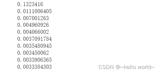
if i%100==0:
print(sess.run(loss,feed_dict={xs:x_data,ys:y_data}))
.
运行结果:
.
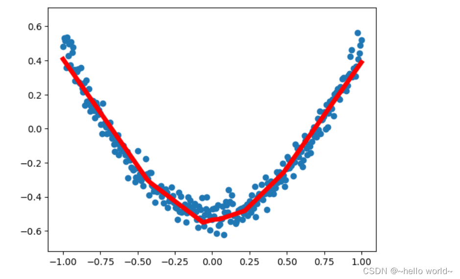
8、结果可视化 plot result
基于已经搭好的神经网络,为方便查看运算进程可将结果可视化
import tensorflow._api.v2.compat.v1 as tf
import numpy as np
import matplotlib.pyplot as plt

#定义一个神经层
def add_layer(inputs,in_size,out_size,activatioin_function=None):
    Weights = tf.Variable(tf.random_normal([in_size,out_size])) #normal distribution是正态分布随机数
    biases = tf.Variable(tf.zeros([1,out_size]) + 0.1) #建议biases不为0,所以加上0.1
    Wx_plus_b = tf.matmul(inputs,Weights) + biases
    #inputs的大小是1*in_size,Weight的大小是in_size*out_size,相乘后大小是1*out_size的行向量
    if activatioin_function is None:
        outputs = Wx_plus_b
    else:
        outputs = activatioin_function(Wx_plus_b)
    return outputs

#生成原始数据
x_data = np.linspace(-1,1,300)[:,np.newaxis].astype('float32')
#在-1到1之间生成300个数的等差数列。
#[:,np.newaxis]加一个维度,使其变成300行,1列的矩阵,
#astype('float32')作为类型转换
noise = np.random.normal(0,0.05,x_data.shape)
y_data = np.square(x_data) - 0.5 + noise

#define placeholder for inputs to network
xs = tf.placeholder(tf.float32,[None,1]) # None代表行和列不固定,1代表只有1列
ys = tf.placeholder(tf.float32,[None,1])

#add hidden layer and output layer
l1 = add_layer(xs,1,10,activatioin_function=tf.nn.relu) #输入层一个神经元,隐藏层10个神经元
prediction = add_layer(l1,10,1,activatioin_function=None)#输出层1个神经元

loss = tf.reduce_mean(tf.reduce_sum(tf.square(ys-prediction),reduction_indices=[1]))
#reduction_indices=[1]是对行方向压缩,按行求和;=[0]是对列方向压缩,按列求和
train_step = tf.train.GradientDescentOptimizer(0.1).minimize(loss)#0.1是学习率

init = tf.global_variables_initializer()
sess = tf.Session()
sess.run(init)

#结果可视化
fig = plt.figure()#生成一个图片框
ax = fig.add_subplot(1,1,1) #连续性的画图需要用ax,一行一列第一个
ax.scatter(x_data,y_data)#以点的形式画出原始数据
plt.ion() #展示动态图或多个窗口,使matplotlib的显示模式转换为交互(interactive)模式。即使在脚本中遇到plt.show(),代码还是会继续执行。
# plt.show()


for i in range(1000):
    #training
    sess.run(train_step,feed_dict={xs:x_data,ys:y_data})#用placeholder,就需要用feed_dict来定义所用到的餐宿
    if i % 50==0 :
  	    # try可以让第一次抹除的时候,若发现没有线段,先跳过这一次
        try:#把这一步提前是为了紧密衔接
            ax.lines.remove(lines[0])  # 去除掉第一个plot
        except Exception:
            pass
        prediction_value = sess.run(prediction,feed_dict={xs: x_data})
        lines = ax.plot(x_data,prediction_value,'r-',lw=5)#红色的线,线的宽度为5
9、优化器
优化器 Optimizer 可以加速神经网络训练,常见的几种优化器:
Stochastic Gradient Descent (SGD)
Momentum
AdaGrad
RMSProp
Adam
一般Adam又快又好
.
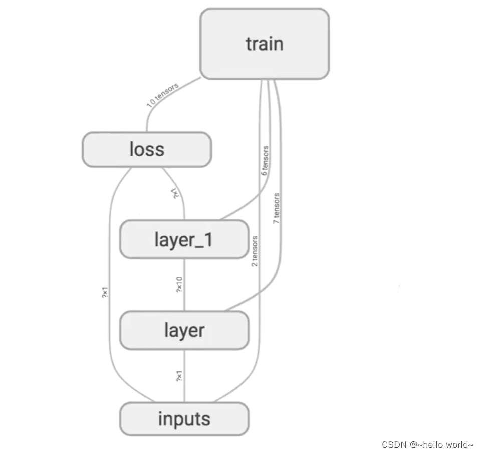
10、网络结构图层可视化
用 Tensorflow 自带的 tensorboard 去可视化所建造出来的神经网络,通过使用这个工具可以很直观的看到整个神经网络的结构、框架。 通常的网络图层整体结构如下图:
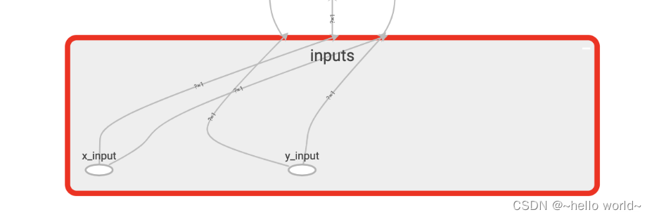
10.1 定义输入
首先从 Input 开始,对于input进行如下修改: 将xs指定名称为x_in,再将ys指定名称y_in,指定的名称将来会在可视化的图层inputs中显示出来。使用with tf.name_scope(‘inputs’)语句可以将xs和ys包含进来,形成一个大的图层,图层的名字就是with tf.name_scope()方法里的参数。
with tf.name_scope('inputs'):
    xs = tfc.placeholder(tf.float32,[None,1],name = 'x_input')
    ys = tfc.placeholder(tf.float32,[None,1],name = 'y_input')
.
with tf.name_scope(‘inputs’)方法构建的inputs神经网络图层:
.
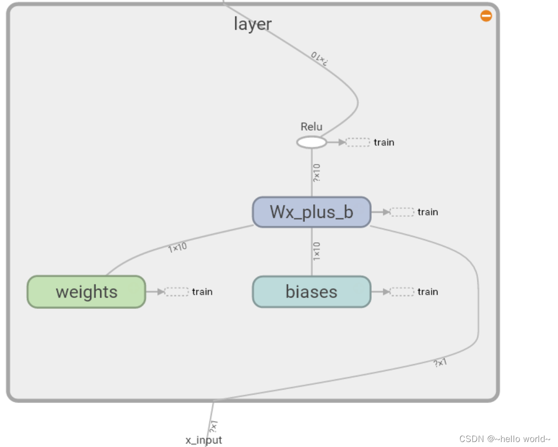
10.2 定义layer层
在定义完大的框架layer之后,需要定义每一个 ’框架‘ 里面的Weights 、biases 和 activation function。 定义的方法同上,使用with tf.name.scope()方法,同时可以在Weights中指定名称W。
def add_layer(inputs,in_size,out_size,activation_function):
    with tf.name_scope('layer'):
        with tf.name_scope('weight'):
            Weights = tf.Variable(tf.random.normal([in_size,out_size]), name='W')
        with tf.name_scope('biases'):
            biases = tf.Variable(tf.zeros([1,out_size])+0.1,name='b')
        with tf.name_scope('Wx_plus_b'):
            Wx_plus_b = tf.add(tf.matmul(inputs,Weights),biases)
        if activation_function is None:
            outputs = Wx_plus_b
        else:
            outputs = activation_function(Wx_plus_b)
        return outputs
.
with tf.name_scope(‘layer’) 方法构建的 layer 神经网络图层:
.
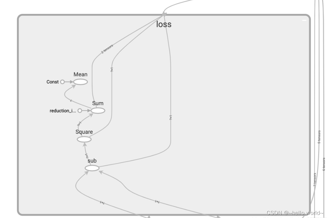
10.3 定义loss层
使用同样的方法,用 with tf.name_scope() 定义 loss 层,并命名为loss。
with tf.name_scope('loss'):
    loss = tf.reduce_mean(tf.reduce_sum(tf.square(ys-prediction), axis=[1]))
.
with tf.name_scope(‘loss’) 方法构建的 loss 神经网络图层:
.
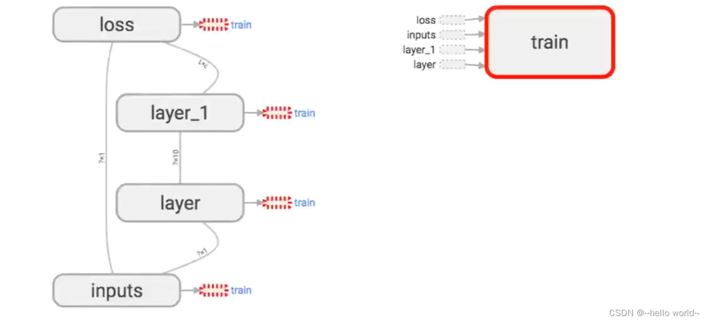
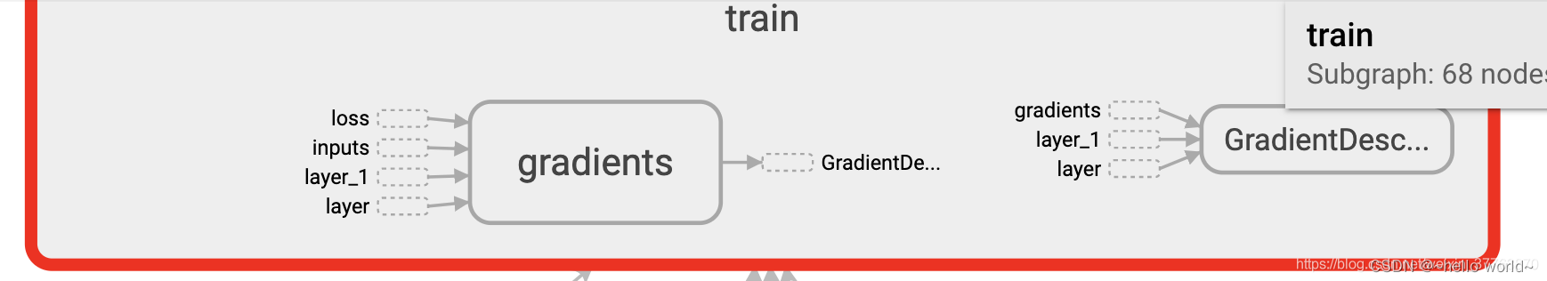
10.4 定义 train 训练层
使用同样的方法,用 with tf.name_scope() 定义train 层。
with tf.name_scope('train'):
    train = tf.compat.v1.train.GradientDescentOptimizer(0.6).minimize(loss)
.
with tf.name_scope(‘train’) 方法构建的 train 神经网络图层:
.
10.5 保存绘制的图到目录
tf.summary.FileWriter() (tf.train.SummaryWriter() 将上面 ‘绘画’ 出的图保存到一个目录中,以方便后期在浏览器中可以浏览。 这个方法中的第二个参数需要使用sess.graph , 因此需要把这句话放在获取session的后面。 这里的graph是将前面定义的框架信息收集起来,然后放在logs/目录下面。
sess = tfc.Session()
writer = tf.compat.v1.summary.FileWriter("logs/", sess.graph)
init = tf.compat.v1.global_variables_initializer()
sess.run(init)
10.6 浏览器查看绘制的图
在终端中 ,使用 $ tensorboard --logdir=‘logs/’,同时将终端中输出的网址复制到浏览器中,便可以看到之前定义的视图框架了。
11、训练过程可视化?
from __future__ import print_function
import tensorflow as tf
import numpy as np
import matplotlib.pyplot as plt
import tensorflow.compat.v1 as tfc
tf.compat.v1.disable_eager_execution()

def add_layer(inputs, in_size, out_size, n_layer, activation_function=None):
    # add one more layer and return the output of this layer
    layer_name = 'layer%s' % n_layer
    with tf.name_scope(layer_name):
        with tf.name_scope('weights'):
            Weights = tf.Variable(tf.random.normal([in_size, out_size]), name='W')
            tf.summary.histogram(layer_name + '/weights', Weights)
        with tf.name_scope('biases'):
            biases = tf.Variable(tf.zeros([1, out_size]) + 0.1, name='b')
            tf.summary.histogram(layer_name + '/biases', biases)
        with tf.name_scope('Wx_plus_b'):
            Wx_plus_b = tf.add(tf.matmul(inputs, Weights), biases)
        if activation_function is None:
            outputs = Wx_plus_b
        else:
            outputs = activation_function(Wx_plus_b, )
        tf.summary.histogram(layer_name + '/outputs', outputs)
    return outputs


# Make up some real data
x_data = np.linspace(-1, 1, 300)[:, np.newaxis]
noise = np.random.normal(0, 0.05, x_data.shape)
y_data = np.square(x_data) - 0.5 + noise

# define placeholder for inputs to network
with tf.name_scope('inputs'):
    xs = tfc.placeholder(tf.float32, [None, 1], name='x_input')
    ys = tfc.placeholder(tf.float32, [None, 1], name='y_input')

# add hidden layer
l1 = add_layer(xs, 1, 10, n_layer=1, activation_function=tf.nn.relu)
# add output layer
prediction = add_layer(l1, 10, 1, n_layer=2, activation_function=None)

# the error between prediciton and real data
with tf.name_scope('loss'):
    loss = tf.reduce_mean(tf.reduce_sum(tf.square(ys-prediction), axis=[1]))
    tf.summary.scalar('loss', loss)

with tf.name_scope('train'):
    train = tf.compat.v1.train.GradientDescentOptimizer(0.6).minimize(loss)

sess = tfc.Session()
merged = tfc.summary.merge_all()

writer = tf.compat.v1.summary.FileWriter("logs/", sess.graph)
init = tf.compat.v1.global_variables_initializer()
sess.run(init)

for i in range(1000):
    sess.run(train, feed_dict={xs: x_data, ys: y_data})
    if i % 50 == 0:
        result = sess.run(merged,feed_dict={xs:x_data,ys:y_data})
#         result = sess.run(merged,feed_dict={xs:x_data,ys:y_data})
        writer.add_summary(result,i)
.
12、分类学习
13、过拟合
过拟合的处理请参考:神经网络:关于模型拟合相关基础学习
dropout 解决过拟合
from __future__ import print_function
import tensorflow as tf
import tensorflow.compat.v1 as tfc
from sklearn.datasets import load_digits
from sklearn.model_selection import train_test_split
from sklearn.preprocessing import LabelBinarizer

# load data
digits = load_digits()
X = digits.data
y = digits.target
y = LabelBinarizer().fit_transform(y)
X_train, X_test, y_train, y_test = train_test_split(X, y, test_size=.3)


def add_layer(inputs, in_size, out_size, layer_name, activation_function=None, ):
    # add one more layer and return the output of this layer
    Weights = tf.Variable(tf.random.normal([in_size, out_size]))
    biases = tf.Variable(tf.zeros([1, out_size]) + 0.1, )
    Wx_plus_b = tf.matmul(inputs, Weights) + biases
    # here to dropout
    Wx_plus_b = tf.nn.dropout(Wx_plus_b, keep_prob)
    if activation_function is None:
        outputs = Wx_plus_b
    else:
        outputs = activation_function(Wx_plus_b, )
    tf.summary.histogram(layer_name + '/outputs', outputs)
    return outputs


# define placeholder for inputs to network
keep_prob = tfc.placeholder(tf.float32)
xs = tfc.placeholder(tf.float32, [None, 64])  # 8x8
ys = tfc.placeholder(tf.float32, [None, 10])

# add output layer
l1 = add_layer(xs, 64, 50, 'l1', activation_function=tf.nn.tanh)
prediction = add_layer(l1, 50, 10, 'l2', activation_function=tf.nn.softmax)

# the loss between prediction and real data
cross_entropy = tf.reduce_mean(-tf.reduce_sum(ys * tfc.log(prediction),axis=[1]))  # loss
tf.summary.scalar('loss', cross_entropy)
train_step = tfc.train.GradientDescentOptimizer(0.5).minimize(cross_entropy)

sess = tfc.Session()
merged = tfc.summary.merge_all()
# summary writer goes in here
train_writer = tfc.summary.FileWriter("logs/train", sess.graph)
test_writer = tfc.summary.FileWriter("logs/test", sess.graph)

# 2017-03-02 if using tensorflow >= 0.12
if int((tf.__version__).split('.')[1]) < 12 and int((tf.__version__).split('.')[0]) < 1:
    init = tfc.initialize_all_variables()
else:
    init = tfc.global_variables_initializer()
sess.run(init)
for i in range(500):
    # here to determine the keeping probability
    sess.run(train_step, feed_dict={xs: X_train, ys: y_train, keep_prob: 0.5})
    if i % 50 == 0:
        # record loss
        train_result = sess.run(merged, feed_dict={xs: X_train, ys: y_train, keep_prob: 1})
        test_result = sess.run(merged, feed_dict={xs: X_test, ys: y_test, keep_prob: 1})
        train_writer.add_summary(train_result, i)
        test_writer.add_summary(test_result, i)
.


 4578
4578


 被折叠的 条评论
为什么被折叠?
被折叠的 条评论
为什么被折叠?
 到【灌水乐园】发言


