


目录
P19-使用Decision Trees建模with Gini and Entropy
P20-使用Random Forests Classifiers(分类器)&Regressor(回归器)两种方式建模
一、随机森林对于离散数据的处理 Random Forest Classifier
缩减特征变量X,对于成百上千特征变量的大数据集有非常重要的意义
二、随机森林对于连续数据的处理 Random Forest for Regression
Feature Scaling(特征缩放/标准化) Scikit-Learn's StandardScaler
Evaluating the Regression Algorithm
K-Nearest Neighbor classifier(KNN)建模 using GridSearchCV
K-Nearest Neighbor classifier(KNN)建模 Using RandomizedSearchCV
Gaussian Naive Bayes建模 with Gaussian Process Classifier
P22-Bagging&Boosting 使用Xgboost(极限梯度提升树)和Gradient Boosting(梯度提升树)建模
P23-K Nearest NeighbourKNN(K最近邻)建模
(3)SVM 对于 direct marketing campaigns (phone calls)数据集的处理
(1)应用Gaussian Naive Bayes预测沉船存活人数
(2)应用Multinomial Naive Bayes处理垃圾邮件
Sklearn Pipeline 老外真的很懒,发明了pipeline替代transform几行代码
P26-Votingclassifier及11种算法全自动建模预测输出结果之完整源代码
Preprocessing using min max scaler
MinMaxScaler和StandardScaler的区别:
P28-Hierarchical Clustering哪些存量客户是新产品的目标用户
P29-DBSCAN聚类(基于密度的空间聚类应用噪声)与K means(K均值)及Hierarchical Clustering(层次聚类)区别
P31-KMeans clustering如何验证K点最佳 silhouette analysis
使用轮廓分析(silhouette analysis)在KMeans聚类中选择簇的数量
P32-无监督学习Principal Component AnalysisPCA精简高维数据(降维)
P19-使用Decision Trees建模with Gini and Entropy
决策树是一种常用的机器学习算法,它的主要原理是通过一系列的问题将数据集进行划分,每个节点代表一个问题,每个分支代表一个答案,最后的每个叶节点代表一个预测结果。
决策树的优点主要包括:
首先,决策树的模型很容易可视化,这使得非专家也能理解其决策过程;
其次,该算法完全不受数据缩放的影响,特征的尺度完全不一样时或者二元特征和连续特征同时存在时,决策树的效果很好;
此外,决策树可以用于小数据集,并且其时间复杂度较小。
最后,值得一提的是,决策树是random forests和gradient boosted tree的基模型,一切高级的树模型都是基于决策树。
然而,决策树也有其缺点:
首先,即使做了预剪枝,决策树也经常会过拟合,泛化性能很差;
其次,在处理大型数据集时,由于必须评估树中每个节点的所有可能拆分,所以计算量会很大。
导入函数库
import numpy as np
import pandas as pd
import matplotlib.pyplot as plt
import seaborn as sns
from sklearn import tree
%matplotlib inline
加载数据集
import ssl
ssl._create_default_https_context = ssl._create_unverified_context
data=sns.load_dataset('iris') 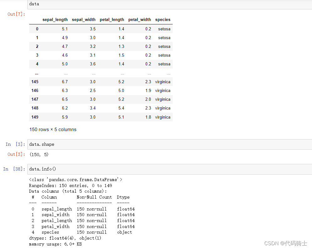
划分特征集和响应集
X = data.drop(['species'], axis=1)
y = data['species']
划分训练集和测试集
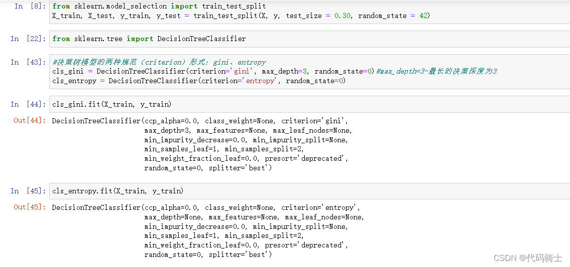
from sklearn.model_selection import train_test_split
X_train, X_test, y_train, y_test = train_test_split(X, y, test_size = 0.30, random_state = 42)
加载决策树算法类
from sklearn.tree import DecisionTreeClassifier使用两种不同的决策树模型规范做训练、预测
#决策树模型的两种规范(criterion)形式:gini、entropy
cls_gini = DecisionTreeClassifier(criterion='gini', max_depth=3, random_state=0)#max_depth=3-最长的决策深度为3
cls_entropy = DecisionTreeClassifier(criterion='entropy', random_state=0)
cls_gini.fit(X_train, y_train)
cls_entropy.fit(X_train, y_train)
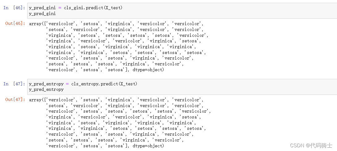
y_pred_gini = cls_gini.predict(X_test)
y_pred_entropy = cls_entropy.predict(X_test)
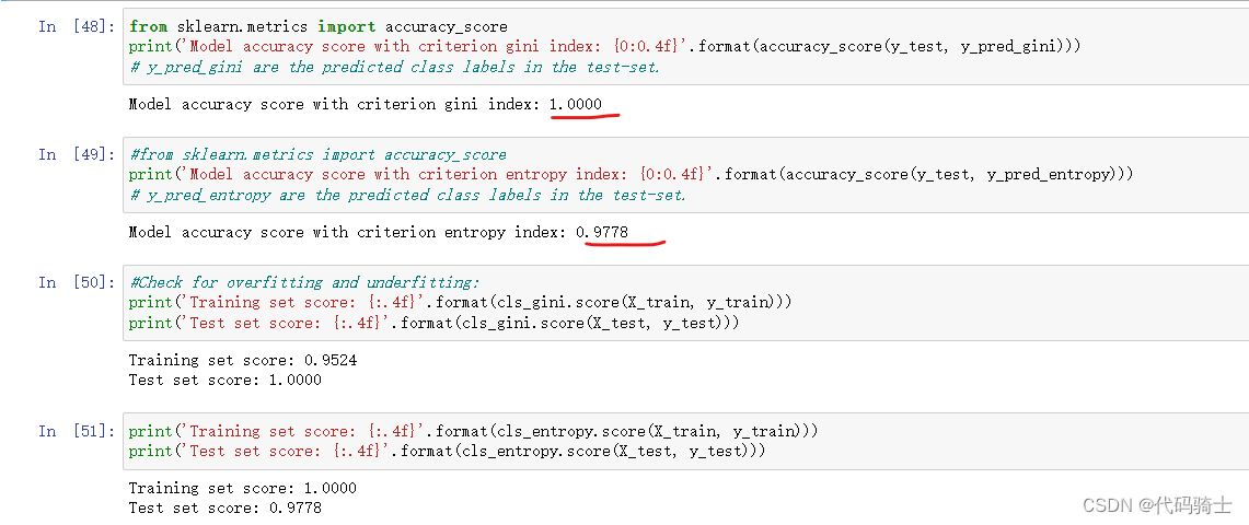
分别求得两种不同决策树的准确值
from sklearn.metrics import accuracy_score
print('Model accuracy score with criterion gini index: {0:0.4f}'.format(accuracy_score(y_test, y_pred_gini)))
# y_pred_gini are the predicted class labels in the test-set.

#from sklearn.metrics import accuracy_score
print('Model accuracy score with criterion entropy index: {0:0.4f}'.format(accuracy_score(y_test, y_pred_entropy)))
# y_pred_entropy are the predicted class labels in the test-set.

#Check for overfitting and underfitting:
print('Training set score: {:.4f}'.format(cls_gini.score(X_train, y_train)))
print('Test set score: {:.4f}'.format(cls_gini.score(X_test, y_test)))

print('Training set score: {:.4f}'.format(cls_entropy.score(X_train, y_train)))
print('Test set score: {:.4f}'.format(cls_entropy.score(X_test, y_test)))
绘制两种不同决策树规范的图像:
#Plot decision tree:
plt.figure(figsize=(12,8))
tree.plot_tree(cls_gini.fit(X_train, y_train))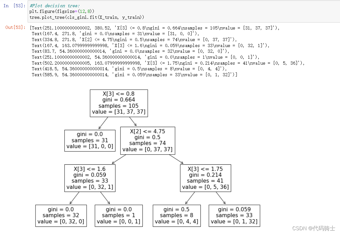
#Plot decision tree:
plt.figure(figsize=(12,8))
tree.plot_tree(cls_entropy.fit(X_train, y_train)) 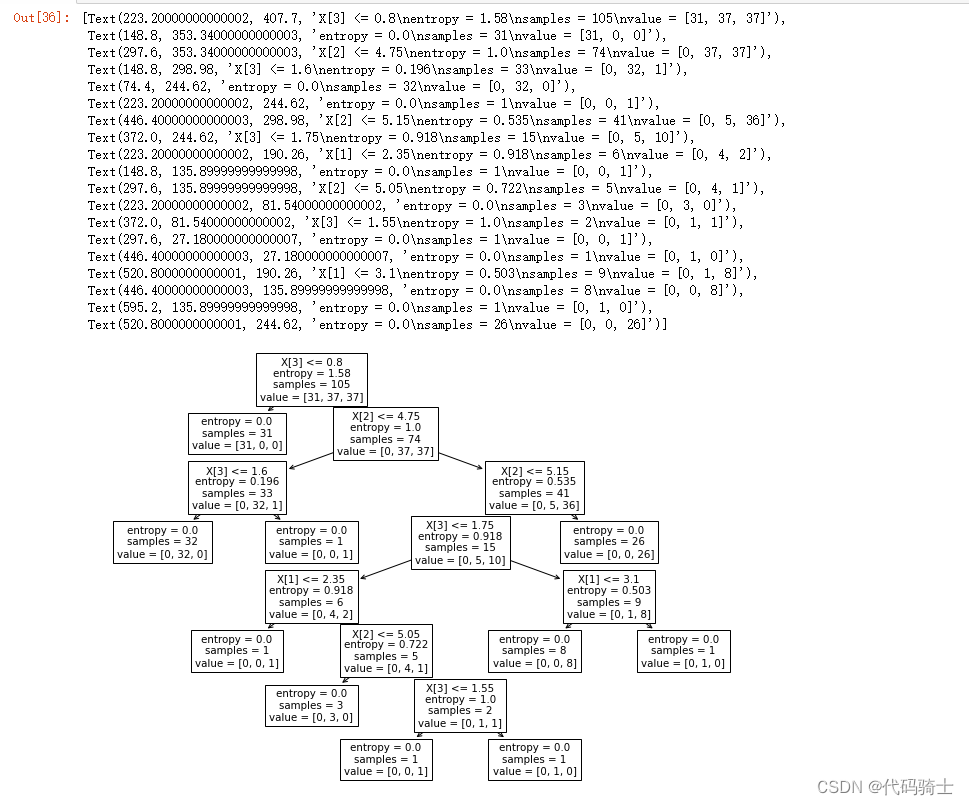
决策树
Gini规范
Entropy规范

P20-使用Random Forests Classifiers(分类器)&Regressor(回归器)两种方式建模
重点:
-Feature_Importances_
-Feature Scaling Scikit-Learn's StandardScaler
-调参随机森林决策树的大小n_estimators
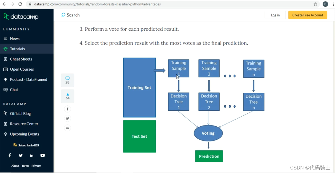
随机森林既可以处理离散量(可以做分类)也可以处理连续量(可以做回归)。
随机森林是一种集成学习方法,它由多个决策树构成,可以用于处理分类和回归问题。这种算法的名字源于它灵活、易用的特性,它可以整合多个决策树的输出以生成单一结果。
每个决策树都是一个基本问题的拆分数据的方法,例如,“我应该去冲浪吗?”然后会有一系列的问题来确定答案,如“海浪涌动的时间很长吗?”或者“风是吹向海面的吗?”这些问题构成决策树中的决策节点。每个问题都有助于个人做出最终决定,最终决定将由叶节点表示。符合条件的观测值将进入“是”分支,而不符合条件的观测值将进入备用路径。
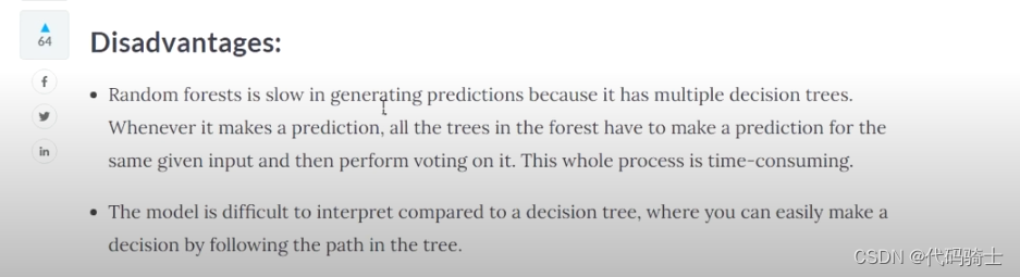
随机森林的优点包括可以在内部进行评估,无偏估计,抗噪能力,抗缺省值等。然而,它的缺点可能包括模型过于复杂,训练时间过长,预测结果的解释性较差等。
在Python中,随机森林的实现可以使用scikit-learn库来完成。总的来说,随机森林是一个强大且灵活的工具,适用于各种机器学习任务。
随机森林是一种高度灵活且对用户友好的机器学习算法,适用于分类和回归任务。以下是随机森林算法的一些主要优点:
1. 表现性能优秀:随机森林算法具有很高的准确性,并且在许多情况下都优于其他算法。
2. 能够处理高维度数据:随机森林不需要进行特征选择或降维处理,它能直接处理含有大量特征的数据集。
3. 抗噪声能力强:随机森林对于噪声数据有优秀的鲁棒性,即使在数据噪音较大的情况下也不容易过拟合。
4. 训练速度快:随机森林的训练过程迅速,并且可以并行化处理,进一步提高训练效率。
5. 提供特征重要性评估:随机森林可以给出各个特征对于预测结果的重要性排序。
6. 能处理缺失值问题:当数据集中存在大量缺失值时,随机森林仍能维持其预测准确性。
7. 可以平衡误差:对于不平衡数据集,随机森林提供了有效的方法来平衡误差。然而,尽管随机森林有许多优点,但也存在一些缺点:
1. 空间和时间需求大:当决策树的数量增加时,为了进行模型训练,所需的存储空间和计算时间也会相应增加。这可能会影响模型在实时性要求较高的应用场景中的使用效率。
2. 可能产生过拟合:虽然随机森林具有较强的抗噪能力,但在数据噪音过大的情况下仍有可能过拟合。

导入函数库
import numpy as np
import pandas as pd
import matplotlib.pyplot as plt
import seaborn as sns
%matplotlib inline
一、随机森林对于离散数据的处理 Random Forest Classifier
加载数据集
data=sns.load_dataset('iris') #参照第19课和第11课
data
查看数据集
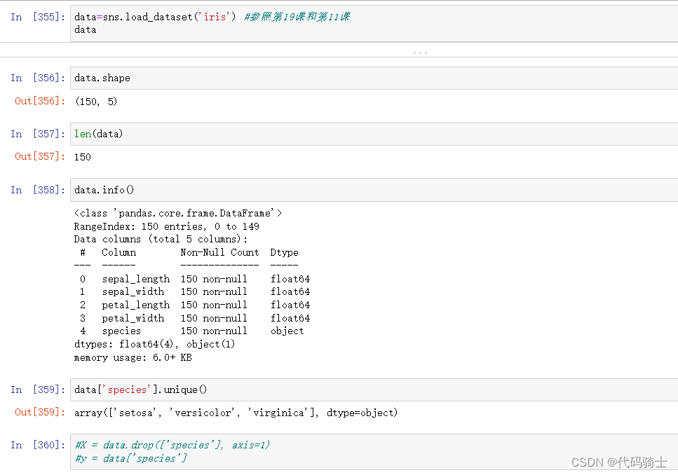
划分特征变量与响应变量
X=data[['sepal_length', 'sepal_width', 'petal_length', 'petal_width']]  # Features
y=data['species']  # Labels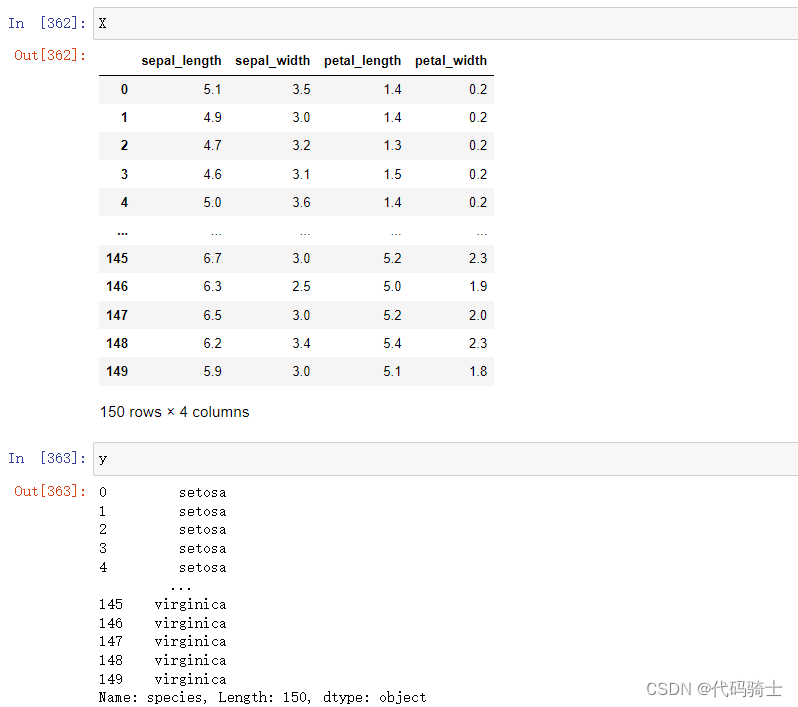
划分训练集和测试集
from sklearn.model_selection import train_test_split
X_train, X_test, y_train, y_test = train_test_split(X, y, test_size = 0.30, random_state = 42)
导入随机森林分类器函数进行模型训练和预测
#Import Random Forest Model
from sklearn.ensemble import RandomForestClassifier

#Create a Gaussian Classifier
clf=RandomForestClassifier(n_estimators=100)#n_estimators=100:用100棵树进行建模

#Train the model using the training sets y_pred=clf.predict(X_test)
clf.fit(X_train,y_train)

y_pred=clf.predict(X_test)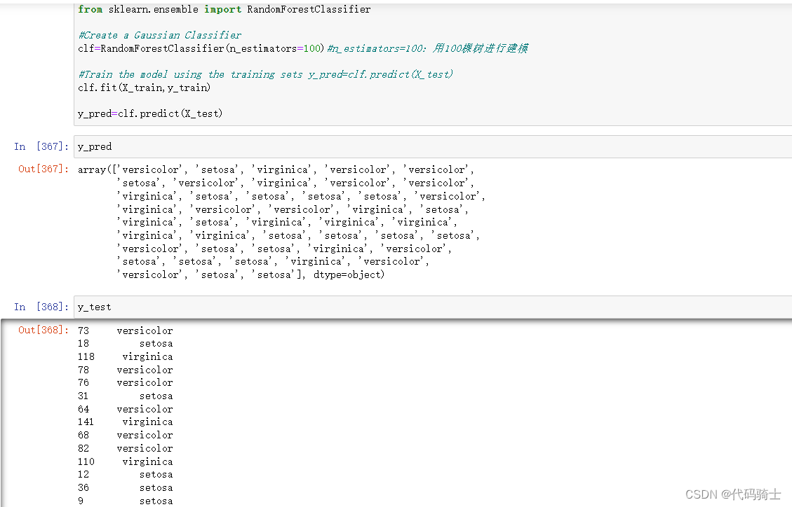
导入metrics库查看随机森林分类模型的准确性
#Import scikit-learn metrics module for accuracy calculation
from sklearn import metrics

# Model Accuracy, how often is the classifier correct?
print("Accuracy:",metrics.accuracy_score(y_test, y_pred))#此方法不能求回归器的准确性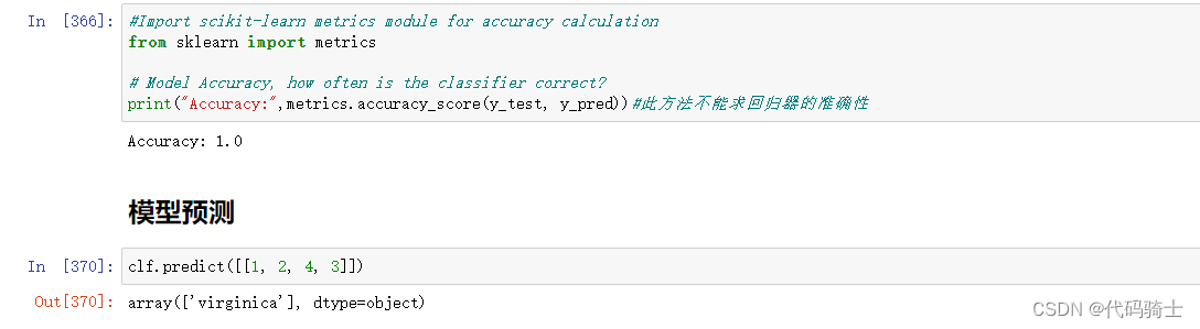
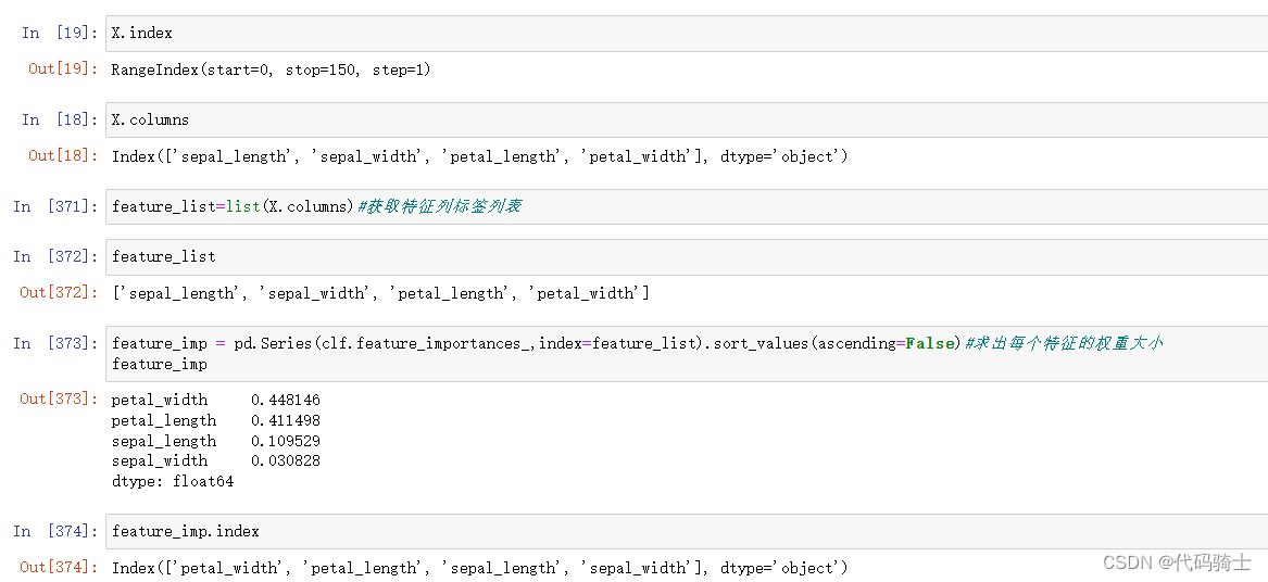
特征变量权重分析 Feature_Importances_
特征变量权重分析(Feature Importances)是一种评估模型中各个特征对预测结果的贡献程度的方法。在机器学习和统计分析中,特征选择和特征工程是非常重要的步骤,因为它们可以帮助我们了解哪些特征对模型的预测性能有显著影响。
特征变量权重分析通常用于以下场景:
-
特征选择:通过计算特征的重要性,我们可以识别出对模型预测性能影响最大的特征,从而减少不必要的特征,提高模型的训练速度和预测性能。
-
特征工程:了解特征的重要性有助于我们进行特征工程,例如创建新的特征、转换现有特征等。
-
解释模型:特征重要性可以帮助我们理解模型是如何根据输入特征进行预测的,从而提高模型的可解释性。
常用的特征变量权重分析方法有:
-
基于树的方法(如决策树、随机森林、梯度提升树等):这些方法通过构建决策树来计算每个特征的重要性。常见的度量标准有基尼系数、信息增益、均方误差等。
-
基于线性模型的方法(如线性回归、逻辑回归等):这些方法通过计算特征的系数来评估其重要性。对于线性模型,特征的系数表示当该特征增加一个单位时,目标变量预期的变化量。
-
基于L1正则化的方法(如Lasso回归):L1正则化会使得一些特征的系数变为零,从而实现特征选择。通过观察被选中的特征,我们可以了解它们的重要性。
-
基于包裹式方法(如递归特征消除、基于遗传算法的特征选择等):这些方法通过反复训练模型并调整特征子集来评估特征的重要性。
总之,特征变量权重分析是一种评估模型中各个特征对预测结果的贡献程度的方法,它可以帮助我们进行特征选择、特征工程和解释模型。
feature_list=list(X.columns)#获取特征列标签列表

feature_imp = pd.Series(clf.feature_importances_,index=feature_list).sort_values(ascending=False)#求出每个特征的权重大小
绘制权重占比图像
# Creating a bar plot
sns.barplot(x=feature_imp, y=feature_imp.index)
# Add labels to your graph
plt.xlabel('Feature Importance Score')
plt.ylabel('Features')
plt.title("Visualizing Important Features")
plt.legend(feature_imp.index)
plt.show()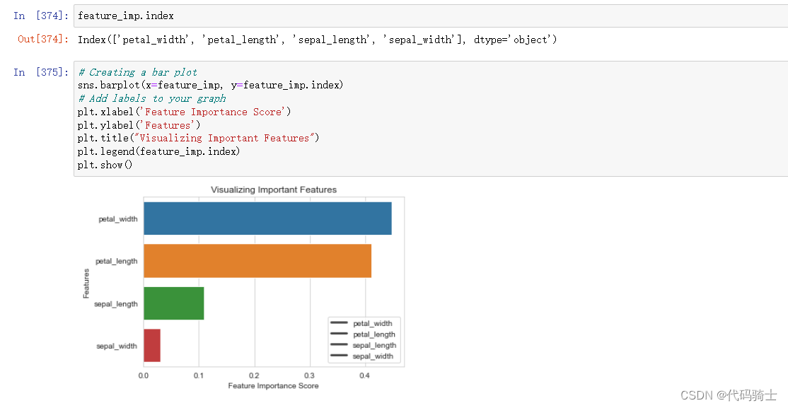
缩减特征变量X,对于成百上千特征变量的大数据集有非常重要的意义
# Split dataset into features and labels
X=data[['petal_length', 'petal_width','sepal_length']]  # Removed feature "sepal width"
y=data['species']
# Split dataset into training set and test set
X_train, X_test, y_train, y_test = train_test_split(X, y, test_size=0.3, random_state=5) # 70% training and 30% test
#Create a Gaussian Classifier
clf=RandomForestClassifier(n_estimators=100)
#Train the model using the training sets y_pred=clf.predict(X_test)
clf.fit(X_train,y_train)
# prediction on test set
y_pred=clf.predict(X_test)
#Import scikit-learn metrics module for accuracy calculation
from sklearn import metrics
# Model Accuracy, how often is the classifier correct?
print("Accuracy:",metrics.accuracy_score(y_test, y_pred))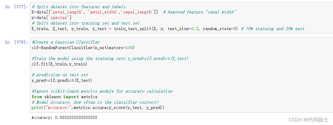
二、随机森林对于连续数据的处理 Random Forest for Regression
dataset = pd.read_csv('./Lesson20-petrol_consumption.csv')
#dataset = pd.read_csv('C:/Users/86185/Desktop/TempDesktop/研究内容/Python学习/Py机深文字教程+源码/LessonPythonCode-main/Lesson20-petrol_consumption.csv')
#C:\Users\86185\Desktop\TempDesktop\研究内容\Python学习\Py机深文字教程+源码\LessonPythonCode-main
#C:/Users/86185/Desktop/TempDesktop/研究内容/Python学习/Py机深文字教程+源码/LessonPythonCode-main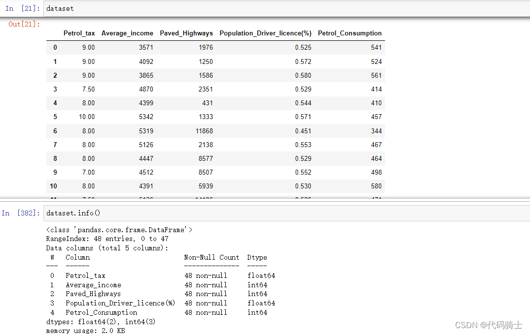
划分特征变量和响应量
X = dataset.iloc[:, 0:4]
y = dataset.iloc[:, 4] 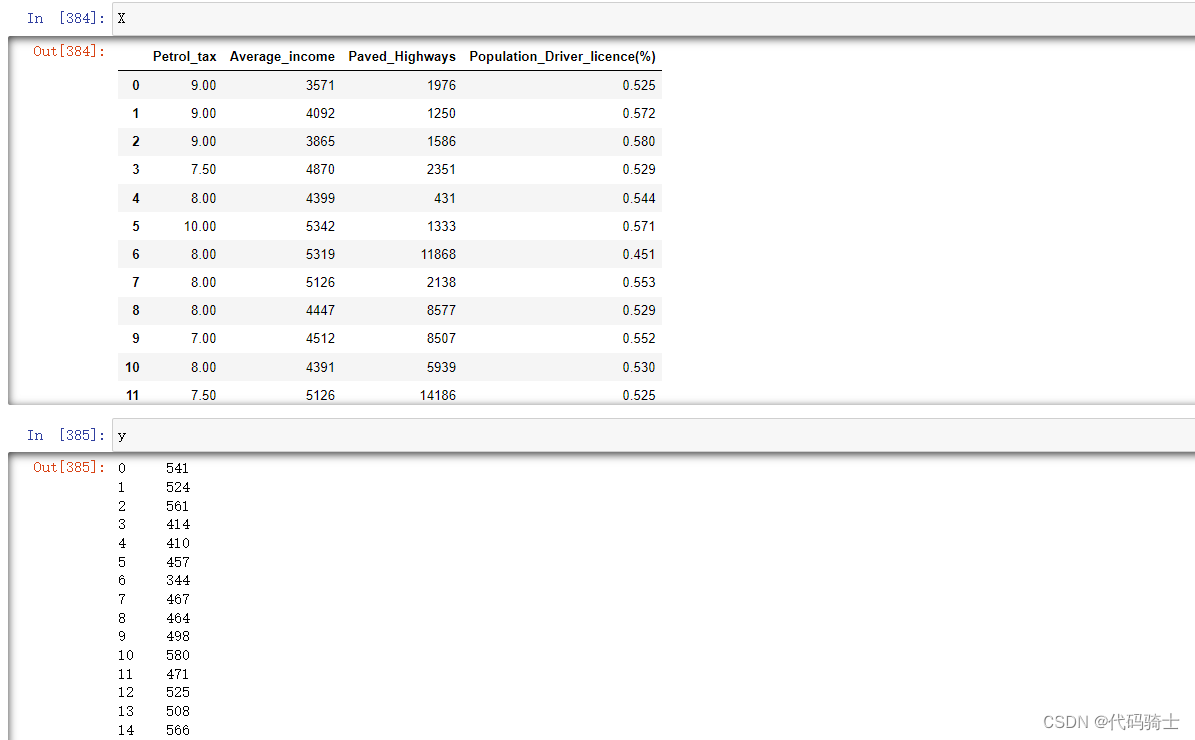
划分训练集和测试集
from sklearn.model_selection import train_test_split

X_train, X_test, y_train, y_test = train_test_split(X, y, test_size=0.2, random_state=0)
Feature Scaling(特征缩放/标准化) Scikit-Learn's StandardScaler
特征标准化:各个特征中数值差异较大,因此直接使用训练的模型效果可能很差,这就需要我们进行特征标准化处理。缩小数据之间的差异,60%的数据值会缩小在-1到1之间。
Petrol_tax——Average_income——Paved_Highways——Population_Driver_licence(%)
9.00—— 3571—— 1976—— 0.525
Feature Scaling(特征缩放)是一种数据预处理技术,用于将不同尺度的特征转换为统一的尺度。这有助于提高机器学习算法的性能和收敛速度。Scikit-Learn是一个流行的Python机器学习库,其中的StandardScaler(标准缩放器)是实现特征缩放的一种方法。
StandardScaler通过计算特征的均值和标准差,将每个特征值减去均值并除以标准差,从而将特征值转换到均值为0、标准差为1的分布上。这种标准化方法使得具有较大尺度的特征对模型的影响减小,从而提高了模型的稳定性和泛化能力。
from sklearn.preprocessing import StandardScaler

sc = StandardScaler()
X_train = sc.fit_transform(X_train)
X_test = sc.transform(X_test)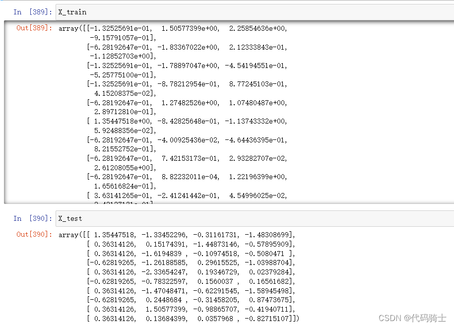
加载模型进行训练与评估
from sklearn.ensemble import RandomForestRegressor

regressor = RandomForestRegressor(n_estimators=100, random_state=0)
regressor.fit(X_train, y_train)
y_pred = regressor.predict(X_test)
Evaluating the Regression Algorithm
from sklearn import metrics

print('Mean Absolute Error:', metrics.mean_absolute_error(y_test, y_pred))
print('Mean Squared Error:', metrics.mean_squared_error(y_test, y_pred))
print('Root Mean Squared Error:', np.sqrt(metrics.mean_squared_error(y_test, y_pred)))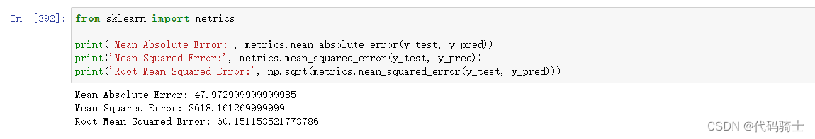
这是机器学习中常用的三种误差度量指标,用于评估模型的预测结果与真实值之间的差异。
-
Mean Absolute Error(平均绝对误差):表示所有样本点上,预测值与真实值的绝对差值的平均数。该指标对异常值比较敏感,因为它会将每个错误都视为相同的重要贡献。
-
Mean Squared Error(均方误差):表示所有样本点上,预测值与真实值的平方差的平均值。相对于平均绝对误差,均方误差对于异常值的影响较小。
-
Root Mean Squared Error(均方根误差):是均方误差的平方根,它衡量了预测值与真实值之间的平均偏差程度。它是衡量回归模型性能的一种常用指标。
在判断回归模型的好坏时,我们通常需要用多个不同的指标来评估整体性能,因为每个指标都有其独特的侧重点和适用情况。以下是根据这三个指标对回归模型进行评估的一般方法:
-
平均绝对误差(Mean Absolute Error, MAE):这个指标衡量了所有样本点上,预测值与真实值的绝对差值的平均数。如果MAE值较小,则说明模型预测的准确性较高;反之,如果MAE值较大,则说明模型预测的准确性较低。不过,需要注意的是,MAE对异常值比较敏感。
-
均方误差(Mean Squared Error, MSE):这个指标衡量了所有样本点上,预测值与真实值的平方差的平均值。如果MSE值较小,则说明模型预测的准确性较高;反之,如果MSE值较大,则说明模型预测的准确性较低。相比于MAE,MSE对于异常值的影响较小。
-
均方根误差(Root Mean Squared Error, RMSE):这是均方误差的平方根,它衡量了预测值与真实值之间的平均偏差程度。如果RMSE值较小,则说明模型预测的准确性较高;反之,如果RMSE值较大,则说明模型预测的准确性较低。
总的来说,我们需要结合使用这些不同的指标,而不是仅仅依赖单一指标来评估模型的性能。同时,我们还需要考虑偏差的风险、错误的大小以及在实践中使用模型时可能产生的影响。此外,通常与基准进行比较也是判断模型好坏的最有效方法。
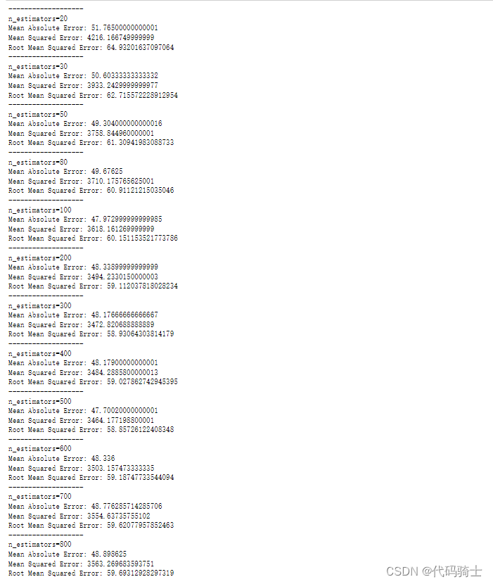
调参随机森林决策树的大小n_estimators
rmse=nestimators=[]
for n in [20,30,50,80,100,200,300,400,500,600,700,800]:
    regressor = RandomForestRegressor(n_estimators=n, random_state=0)
    regressor.fit(X_train, y_train)
    y_pred = regressor.predict(X_test)
    print('-------------------')
    print('n_estimators={}'.format(n))
    print('Mean Absolute Error:', metrics.mean_absolute_error(y_test, y_pred))
    print('Mean Squared Error:', metrics.mean_squared_error(y_test, y_pred))
    print('Root Mean Squared Error:', np.sqrt(metrics.mean_squared_error(y_test, y_pred)))
    rmse=np.append(rmse,np.sqrt(metrics.mean_squared_error(y_test, y_pred)))
    nestimators=np.append(nestimators,n)
通过遍历寻找合适的 n_estimators 参数值(默认是100)
直观显示参数与误差之间的关系(寻找一个误差y最小时的参数x)
# Creating a bar plot
sns.set_style('whitegrid')
plt.plot(nestimators,rmse,'ro',linestyle='dashed',linewidth=1,markersize=10)
# Add labels to your graph
plt.xlabel('Feature Importance Score')
plt.ylabel('Features')
plt.title("Visualizing Important Features/RMSE")
plt.show()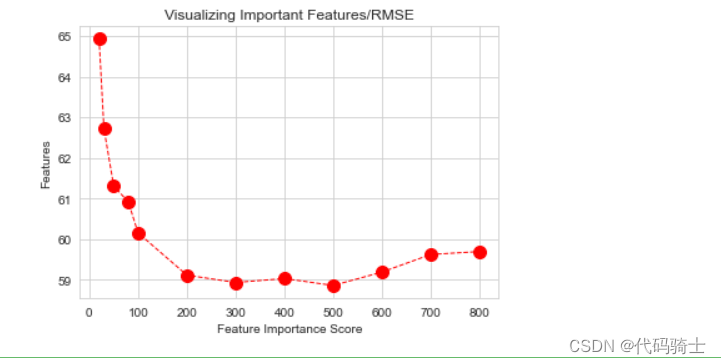
P21-使用Adaboost建模及工作环境下的数据分析整理
https://www.youtube.com/watch?v=1_3s_hwiCO4&list=PLGkfh2EpdoKU3OssXkTl3y7c9tw7jjvHm&index=25
Adaboost,英文全称"Adaptive Boosting",意为自适应增强,是一种基于Boosting集成学习的算法。Boosting是一种试图从多个弱分类器中创建一个强分类器的集合技术。Adaboost的核心思想是通过从训练数据构建模型,然后创建第二个模型来尝试修正第一个模型的错误。
Adaboost算法最初由Yoav Freund和Robert Schapire在1995年提出。该算法的主要目标是通过反复学习不断改变训练样本的权重和弱分类器的权值,最终筛选出权值系数最小的弱分类器组合成一个最终强分类器。
Adaboost,全称为Adaptive Boosting,是一种有效且实用的Boosting算法。它的核心思想是以一种高度自适应的方式按顺序训练弱学习器,针对分类问题,根据前一次的分类效果调整数据的权重。
具体来说,Adaboost算法可以简述为以下三个步骤:
1. 初始化训练数据的权值分布。假设有N个训练样本数据,每一个训练样本最开始时,都被赋予相同的权值:w1=1/N。
2. 训练弱分类器hi。在训练过程中,如果某个训练样本点被弱分类器hi准确地分类,那么在构造下一个训练集中,它对应的权值要减小;相反,如果某个训练样本点被错误分类,那么它的权值就应该增大。权值更新过的样本集被用于训练下一个分类器,整个训练过程如此迭代地进行下去。
3. 将各个训练得到的弱分类器组合成一个强分类器。各个弱分类器的训练过程结束后,加大分类误差率小的弱分类器的权重,使其在最终的分类函数中起着较大的决定作用,而降低分类误差率大的弱分类器的权重,使其在最终的分类函数中起着较小的决定作用。此外,Adaboost也是一种加法模型的学习算法,其损失函数为指数函数。通过不断重复调整权重和训练弱学习器,直到误分类数低于预设值或迭代次数达到指定最大值,最终得到一个强学习器。值得一提的是,Adaboost具有很高的精度,并且充分考虑了每个分类器的权重。但是,Adaboost迭代次数也就是弱分类器数目不太好设定,可以使用交叉验证来进行确定。
adaboost与random forest的区别
Adaboost和Random Forest都是集成学习的算法,然而它们在许多方面存在显著的差异。首先,Adaboost是一种基于Boosting的加法模型学习算法,它反复进行学习,不断调整训练样本的权重和弱分类器的权值,最终选取权值系数最小的弱分类器组合成一个强分类器。其常用的弱学习器是决策树和神经网络。
另一方面,随机森林也是一种集成学习的算法,但它属于Bagging流派。随机森林通过建立并结合多个决策树的输出来得到一个最终结果,这旨在提高预测的准确性。不同于Adaboost一次只使用一个弱分类器,随机森林允许同时使用所有的决策树,并且每棵树的建立都考虑了样本随机性和特征随机性,这样可以减少过拟合的风险。
总结来说,虽然Adaboost和Random Forest都是集成学习的算法,但它们在建模方法、基学习器的选择等方面存在明显的区别。
Boosting与Bagging流派区别
Bagging和Boosting都是将已有的分类或回归算法通过一定方式组合起来,形成一个性能更加强大的分类器。虽然二者都是集成学习的方法,但是存在一些显著的差异。
Bagging,也称为套袋法,其算法过程如下:从原始样本集中抽取训练集。每轮从原始样本集中使用Bootstraping的方法抽取n个训练样本(在训练集中,有些样本可能被多次抽取到,而有些样本可能一次都没有被抽中)。共进行k轮抽取,得到k个训练集。(k个训练集之间是相互独立的) 每次使用一个训练集得到一个模型,k个训练集共得到k个模型。对分类问题:将上步得到的k个模型采用投票的方式得到分类结果;对回归问题,计算上述模型的均值作为最后的结果。(所有模型的重要性相同)。
而Boosting的主要思想是将弱分类器组装成一个强分类器。在PAC(概率近似正确)学习框架下,则一定可以将弱分类器组装成一个强分类器。关于Boosting有两个核心问题: 1. 在每一轮如何改变训练数据的权值或概率分布?通过提高那些在前一轮被弱分类器分错样例的权值,减小前一轮分对样例的权值,来使得分类器重点关注那些被误分的数据,直至所有的样本都被正确分类。2. 通过什么方式来组合弱分类器?通过加法模型将弱分类器进行线性组合,比如AdaBoost通过加权多数表决的方式,即增大错误率小的分类器的权值,同时减小错误率较大的分类器的权值。
从以上描述可以看出,Bagging和Boosting两个流派的区别主要体现在以下几个方面:样本选择、样例权重、预测函数、并行计算以及思路。

为了更好的在编译器中显示图片需要安装python第三方库:
pip install ipython
# pip install ipython

from IPython.display import Image
Image(filename='C:\\Users\\86185\\Desktop\\TempDesktop\\研究内容\\Python学习\\Py机深文字教程+源码\\LessonPythonCode-main\\Lesson21-adaboost.jpg')
#C:\Users\86185\Desktop\TempDesktop\研究内容\Python学习\Py机深文字教程+源码\LessonPythonCode-main
#Image(filename='D:/python/Project0-Python-MachineLearning/Lesson21-adaboost.jpg')
Adaboost算法图解
泰坦尼克号分析(工作环境)
import pandas as pd
import numpy as np
from matplotlib import pyplot as plt
import seaborn as sns
%matplotlib inline

import warnings ## importing warnings library.
warnings.filterwarnings('ignore') ## Ignore warning

import os ## imporing os
print(os.listdir("./"))
## Importing Titanic datasets from www.kaggle.com
train = pd.read_csv("./Lesson21-titanic_train.csv")
test = pd.read_csv("./Lesson21-titanic_test.csv")
#./seaborn-data/raw/titanic
#train = pd.read_csv("./titanic/Lesson21-titanic_train.csv")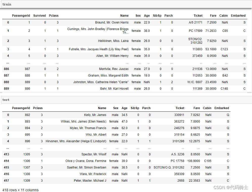
Python可以引入任何图形及图形可视化工具
#导入一个HTML数据分析网页
%%HTML
<div class='tableauPlaceholder' id='viz1516349898238' style='position: relative'><noscript><a href='#'><img alt='An Overview of Titanic Training Dataset ' src='https://public.tableau.com/static/images/Ti/Titanic_data_mining/Dashboard1/1_rss.png' style='border: none' /></a></noscript><object class='tableauViz' style='display:none;'><param name='host_url' value='https%3A%2F%2Fpublic.tableau.com%2F' /> <param name='embed_code_version' value='3' /> <param name='site_root' value='' /><param name='name' value='Titanic_data_mining/Dashboard1' /><param name='tabs' value='no' /><param name='toolbar' value='yes' /><param name='static_image' value='https://public.tableau.com/static/images/Ti/Titanic_data_mining/Dashboard1/1.png' /> <param name='animate_transition' value='yes' /><param name='display_static_image' value='yes' /><param name='display_spinner' value='yes' /><param name='display_overlay' value='yes' /><param name='display_count' value='yes' /><param name='filter' value='publish=yes' /></object></div> <script type='text/javascript'> var divElement = document.getElementById('viz1516349898238'); var vizElement = divElement.getElementsByTagName('object')[0]; vizElement.style.width='100%';vizElement.style.height=(divElement.offsetWidth*0.75)+'px'; var scriptElement = document.createElement('script'); scriptElement.src = 'https://public.tableau.com/javascripts/api/viz_v1.js'; vizElement.parentNode.insertBefore(scriptElement, vizElement); </script>
passengerid = test.PassengerId

print (train.info())
print ("*"*80)
print (test.info())
<class 'pandas.core.frame.DataFrame'> RangeIndex: 891 entries, 0 to 890 Data columns (total 12 columns): # Column Non-Null Count Dtype --- ------ -------------- ----- 0 PassengerId 891 non-null int64 1 Survived 891 non-null int64 2 Pclass 891 non-null int64 3 Name 891 non-null object 4 Sex 891 non-null object 5 Age 714 non-null float64 6 SibSp 891 non-null int64 7 Parch 891 non-null int64 8 Ticket 891 non-null object 9 Fare 891 non-null float64 10 Cabin 204 non-null object 11 Embarked 889 non-null object dtypes: float64(2), int64(5), object(5) memory usage: 83.7+ KB None ******************************************************************************** <class 'pandas.core.frame.DataFrame'> RangeIndex: 418 entries, 0 to 417 Data columns (total 11 columns): # Column Non-Null Count Dtype --- ------ -------------- ----- 0 PassengerId 418 non-null int64 1 Pclass 418 non-null int64 2 Name 418 non-null object 3 Sex 418 non-null object 4 Age 332 non-null float64 5 SibSp 418 non-null int64 6 Parch 418 non-null int64 7 Ticket 418 non-null object 8 Fare 417 non-null float64 9 Cabin 91 non-null object 10 Embarked 418 non-null object dtypes: float64(2), int64(4), object(5) memory usage: 36.0+ KB None
写个小程序统计缺失值
# total percentage of the missing values
# 统计缺失值
def missing_percentage(df):
    """This function takes a DataFrame(df) as input and returns two columns, total missing values and total missing values percentage"""
    total = df.isnull().sum().sort_values(ascending = False)
    percent = round(df.isnull().sum().sort_values(ascending = False)/len(df)*100,2)
    return pd.concat([total, percent], axis=1, keys=['Total','Percent'])
missing_percentage(train)
missing_percentage(test)
def percent_value_counts(df, feature):
    percent = pd.DataFrame(round(df.loc[:,feature].value_counts(dropna=False, normalize=True)*100,2))
    ## creating a df with th
    total = pd.DataFrame(df.loc[:,feature].value_counts(dropna=False))
    ## concating percent and total dataframe

    total.columns = ["Total"]
    percent.columns = ['Percent']
    return pd.concat([total, percent], axis = 1)
percent_value_counts(train, 'Embarked')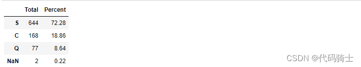
train[train.Embarked.isnull()]
sns.set_style('darkgrid')
fig, ax = plt.subplots(figsize=(16,12),ncols=2)
ax1 = sns.boxplot(x="Embarked", y="Fare", hue="Pclass", data=train, ax = ax[0]);
ax2 = sns.boxplot(x="Embarked", y="Fare", hue="Pclass", data=test, ax = ax[1]);
ax1.set_title("Training Set", fontsize = 18)
ax2.set_title('Test Set',  fontsize = 18)


## Fixing legends
leg_1 = ax1.get_legend()
leg_1.set_title("PClass")
legs = leg_1.texts
legs[0].set_text('Upper')
legs[1].set_text('Middle')
legs[2].set_text('Lower')

fig.show()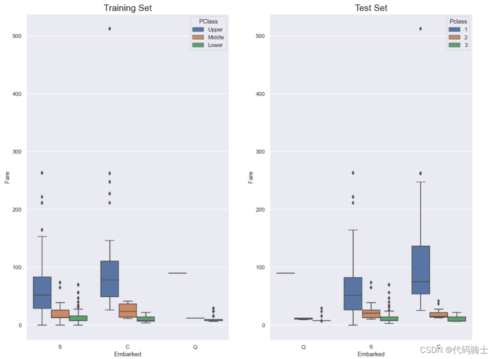
Here, in both training set and test set, the average fare closest to $80 are in the C Embarked values where pclass is 1. So, let's fill in the missing values as "C"
在这里,训练集和测试集中平均票价最接近80美元的乘客登船地点(C Embarked)值都是pclass为1。因此,让我们将缺失值填充为“C”
## Replacing the null values in the Embarked column with the mode.
train.Embarked.fillna("C", inplace=True)
print("Train Cabin missing: " + str(train.Cabin.isnull().sum()/len(train.Cabin)))
print("Test Cabin missing: " + str(test.Cabin.isnull().sum()/len(test.Cabin)))Train Cabin missing: 0.7710437710437711 Test Cabin missing: 0.7822966507177034
## Concat train and test into a variable "all_data"
survivers = train.Survived

train.drop(["Survived"],axis=1, inplace=True)

all_data = pd.concat([train,test], ignore_index=False)

## Assign all the null values to N
all_data.Cabin.fillna("N", inplace=True)
all_data.Cabin = [i[0] for i in all_data.Cabin]percent_value_counts(all_data, "Cabin")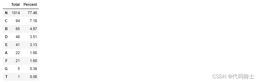
all_data.groupby("Cabin")['Fare'].mean().sort_values()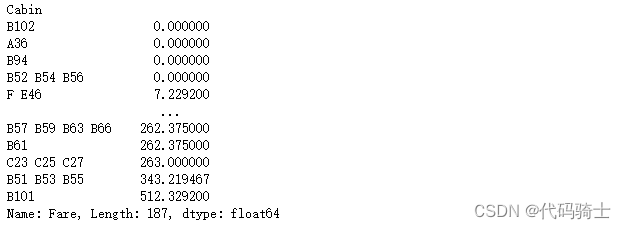
def cabin_estimator(i):
    """Grouping cabin feature by the first letter"""
    a = 0
    if i<16:
        a = "G"
    elif i>=16 and i<27:
        a = "F"
    elif i>=27 and i<38:
        a = "T"
    elif i>=38 and i<47:
        a = "A"
    elif i>= 47 and i<53:
        a = "E"
    elif i>= 53 and i<54:
        a = "D"
    elif i>=54 and i<116:
        a = 'C'
    else:
        a = "B"
    return a
with_N = all_data[all_data.Cabin == "N"]

without_N = all_data[all_data.Cabin != "N"]
##applying cabin estimator function.
with_N['Cabin'] = with_N.Fare.apply(lambda x: cabin_estimator(x))
## getting back train.
all_data = pd.concat([with_N, without_N], axis=0)
## PassengerId helps us separate train and test.
all_data.sort_values(by = 'PassengerId', inplace=True)
## Separating train and test from all_data.
train = all_data[:891]
test = all_data[891:]
# adding saved target variable with train.
train['Survived'] = survivers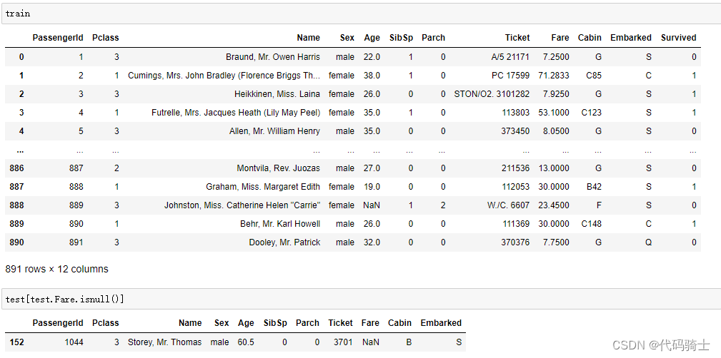
missing_value = test[(test.Pclass == 3) &
                     (test.Embarked == "S") &
                     (test.Sex == "male")].Fare.mean()
## replace the test.fare null values with test.fare mean
test.Fare.fillna(missing_value, inplace=True)missing_value12.718872
test[test.Fare.isnull()]Passenger Id Pclass Name Sex Age SibSpParch Ticket Fare Cabin Embarked
print ("Train age missing value: " + str((train.Age.isnull().sum()/len(train))*100)+str("%"))
print ("Test age missing value: " + str((test.Age.isnull().sum()/len(test))*100)+str("%"))
Train age missing value: 19.865319865319865% Test age missing value: 20.574162679425836%
import seaborn as sns
pal = {'male':"green", 'female':"Pink"}
sns.set(style="darkgrid")
plt.subplots(figsize = (15,8))
ax = sns.barplot(x = "Sex",
                 y = "Survived",
                 data=train,
                 palette = pal,
                 linewidth=5,
                 order = ['female','male'],
                 capsize = .05,

                )

plt.title("Survived/Non-Survived Passenger Gender Distribution", fontsize = 25,loc = 'center', pad = 40)
plt.ylabel("% of passenger survived", fontsize = 15, )
plt.xlabel("Sex",fontsize = 15);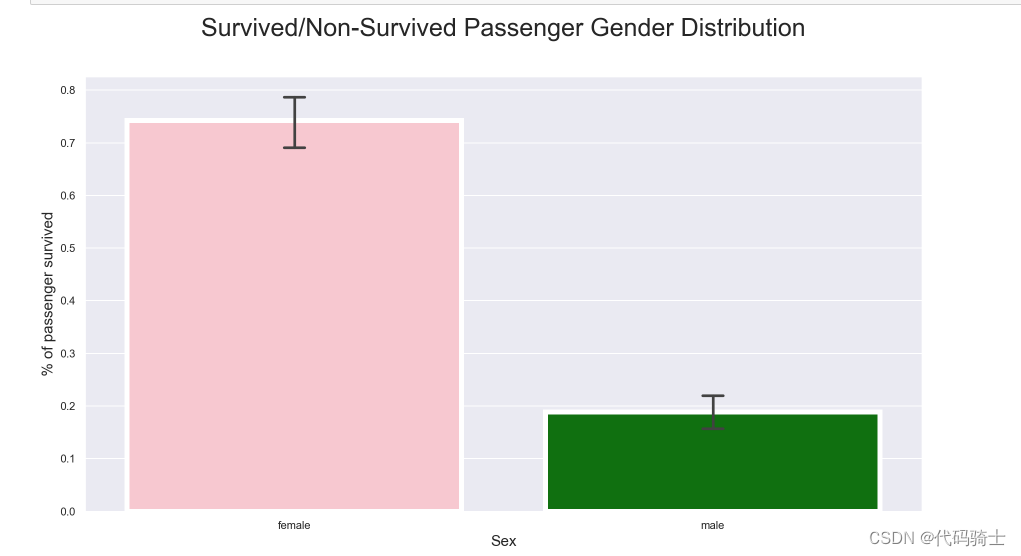
pal = {1:"seagreen", 0:"gray"}
sns.set(style="darkgrid")
plt.subplots(figsize = (15,8))
ax = sns.countplot(x = "Sex",
                   hue="Survived",
                   data = train,
                   linewidth=4,
                   palette = pal
)

## Fixing title, xlabel and ylabel
plt.title("Passenger Gender Distribution - Survived vs Not-survived", fontsize = 25, pad=40)
plt.xlabel("Sex", fontsize = 15);
plt.ylabel("# of Passenger Survived", fontsize = 15)

## Fixing xticks
#labels = ['Female', 'Male']
#plt.xticks(sorted(train.Sex.unique()), labels)

## Fixing legends
leg = ax.get_legend()
leg.set_title("Survived")
legs = leg.texts
legs[0].set_text("No")
legs[1].set_text("Yes")
plt.show()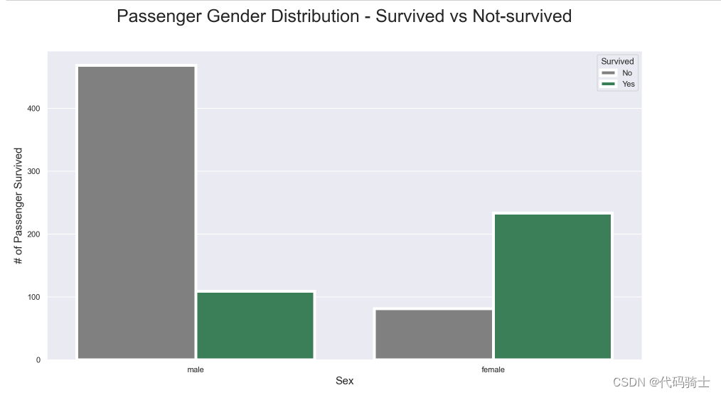
temp = train[['Pclass', 'Survived', 'PassengerId']].groupby(['Pclass', 'Survived']).count().reset_index()
temp_df = pd.pivot_table(temp, values = 'PassengerId', index = 'Pclass',columns = 'Survived')
names = ['No', 'Yes']
temp_df.columns = names
r = [0,1,2]
totals = [i+j for i, j in zip(temp_df['No'], temp_df['Yes'])]
No_s = [i / j * 100 for i,j in zip(temp_df['No'], totals)]
Yes_s = [i / j * 100 for i,j in zip(temp_df['Yes'], totals)]
## Plotting
plt.subplots(figsize = (15,10))
barWidth = 0.60
names = ('Upper', 'Middle', 'Lower')
# Create green Bars
plt.bar(r, No_s, color='Red', edgecolor='white', width=barWidth)
# Create orange Bars
plt.bar(r, Yes_s, bottom=No_s, color='Green', edgecolor='white', width=barWidth)


# Custom x axis
plt.xticks(r, names)
plt.xlabel("Pclass")
plt.ylabel('Percentage')

# Show graphic
plt.show()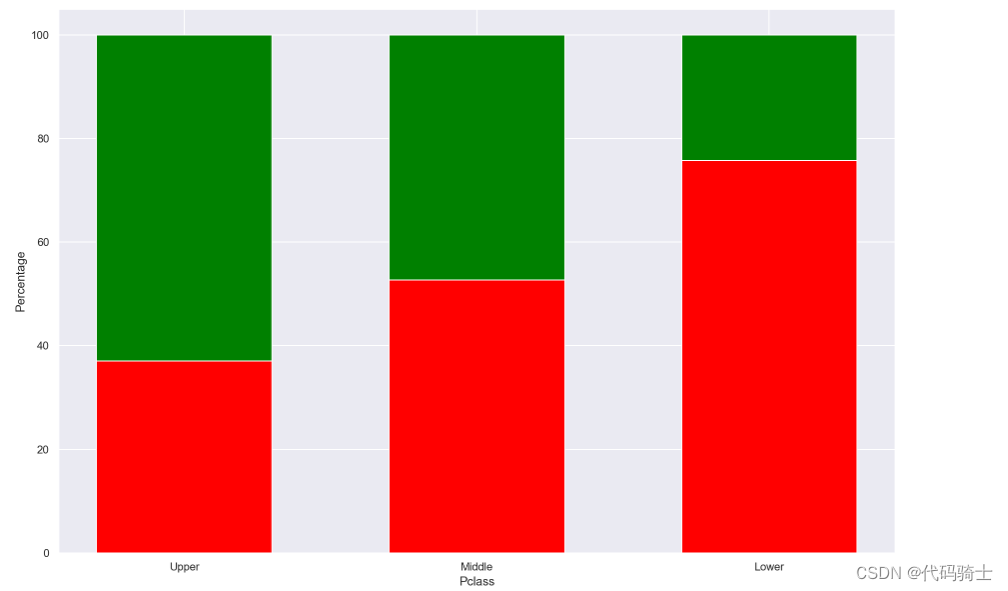
plt.subplots(figsize = (15,10))
sns.barplot(x = "Pclass",
            y = "Survived",
            data=train,
            linewidth=6,
            capsize = .05,
            errcolor='blue',
            errwidth = 3


           )
plt.title("Passenger Class Distribution - Survived vs Non-Survived", fontsize = 25, pad=40)
plt.xlabel("Socio-Economic class", fontsize = 15);
plt.ylabel("% of Passenger Survived", fontsize = 15);
names = ['Upper', 'Middle', 'Lower']
#val = sorted(train.Pclass.unique())
val = [0,1,2] ## this is just a temporary trick to get the label right.
plt.xticks(val, names);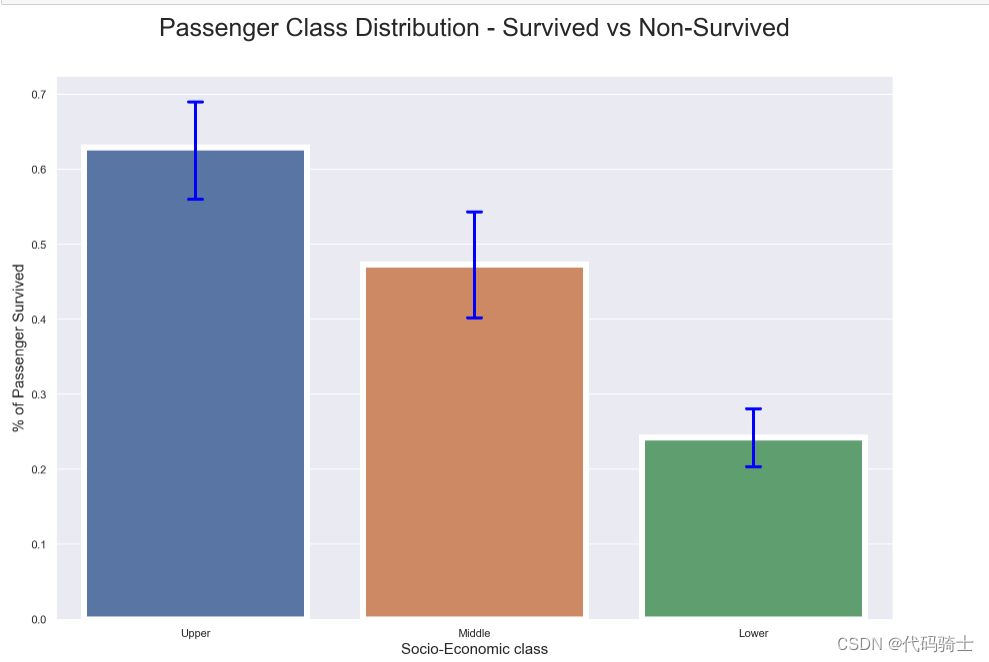
# Kernel Density Plot
fig = plt.figure(figsize=(15,8),)
## I have included to different ways to code a plot below, choose the one that suites you.
ax=sns.kdeplot(train.Pclass[train.Survived == 0] ,
               color='blue',
               shade=True,
               label='not survived')
ax=sns.kdeplot(train.loc[(train['Survived'] == 1),'Pclass'] ,
               color='g',
               shade=True,
               label='survived',
              )
plt.title('Passenger Class Distribution - Survived vs Non-Survived', fontsize = 25, pad = 40)
plt.ylabel("Frequency of Passenger Survived", fontsize = 15, labelpad = 20)
plt.xlabel("Passenger Class", fontsize = 15,labelpad =20)
## Converting xticks into words for better understanding
labels = ['Upper', 'Middle', 'Lower']
plt.xticks(sorted(train.Pclass.unique()), labels);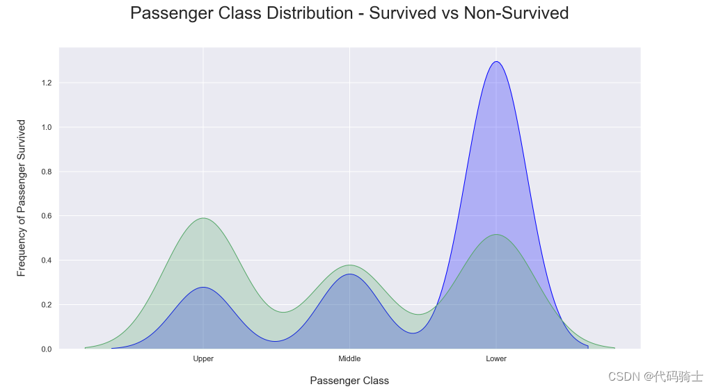
# Kernel Density Plot
fig = plt.figure(figsize=(15,8),)
ax=sns.kdeplot(train.loc[(train['Survived'] == 0),'Fare'] , color='blue',shade=True,label='not survived')
ax=sns.kdeplot(train.loc[(train['Survived'] == 1),'Fare'] , color='g',shade=True, label='survived')
plt.title('Fare Distribution Survived vs Non Survived', fontsize = 25, pad = 40)
plt.ylabel("Frequency of Passenger Survived", fontsize = 15, labelpad = 20)
plt.xlabel("Fare", fontsize = 15, labelpad = 20);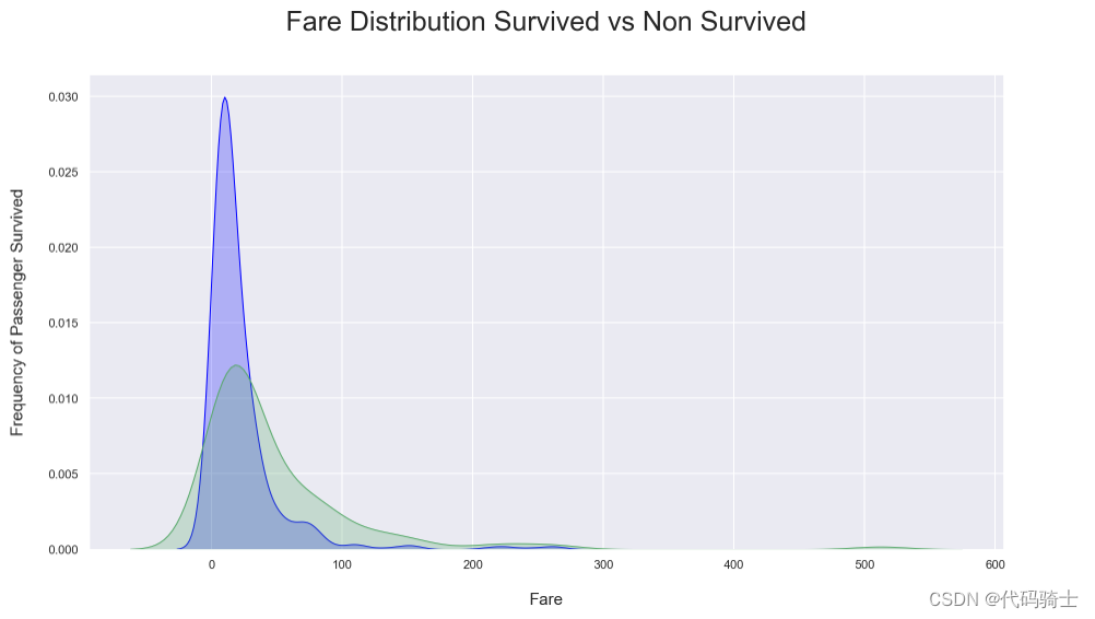
train[train.Fare > 280]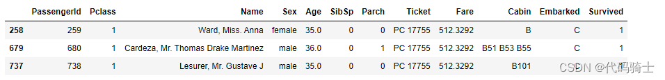
# Kernel Density Plot
fig = plt.figure(figsize=(15,8),)
ax=sns.kdeplot(train.loc[(train['Survived'] == 0),'Age'] , color='blue',shade=True,label='not survived')
ax=sns.kdeplot(train.loc[(train['Survived'] == 1),'Age'] , color='g',shade=True, label='survived')
plt.title('Age Distribution - Surviver V.S. Non Survivors', fontsize = 25, pad = 40)
plt.xlabel("Age", fontsize = 15, labelpad = 20)
plt.ylabel('Frequency', fontsize = 15, labelpad= 20);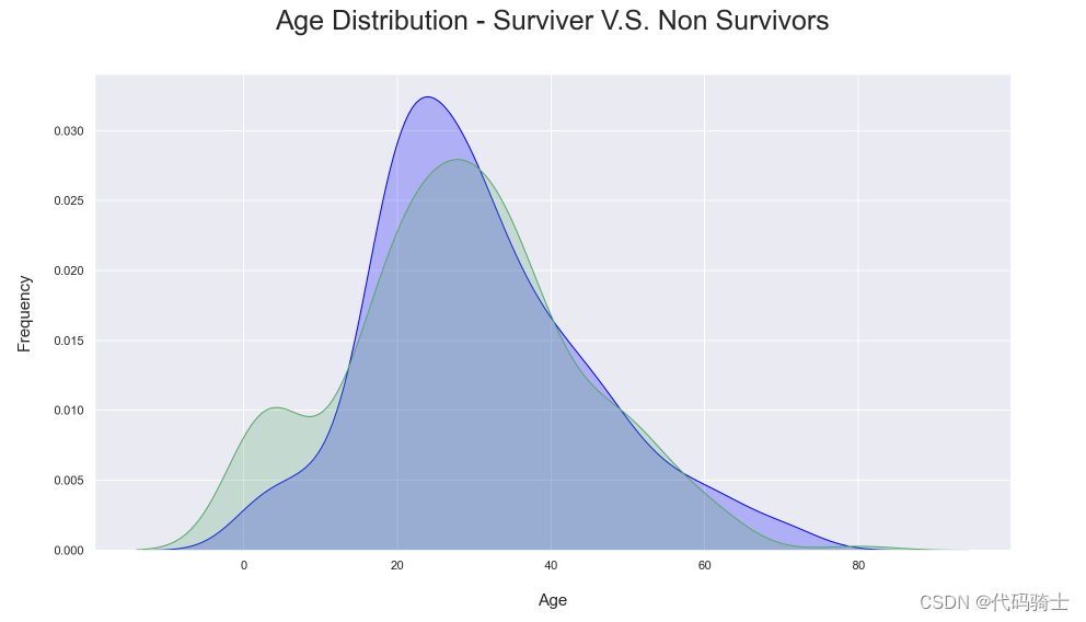
pal = {1:"seagreen", 0:"gray"}
g = sns.FacetGrid(train,size=5, col="Sex", row="Survived", margin_titles=True, hue = "Survived",
                  palette=pal)
g = g.map(plt.hist, "Age", edgecolor = 'white');
g.fig.suptitle("Survived by Sex and Age", size = 25)
plt.subplots_adjust(top=0.90)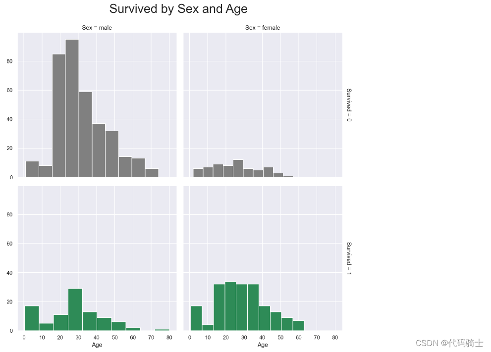
g = sns.FacetGrid(train,size=5, col="Sex", row="Embarked", margin_titles=True, hue = "Survived",
                  palette = pal
                  )
g = g.map(plt.hist, "Age", edgecolor = 'white').add_legend();
g.fig.suptitle("Survived by Sex and Age", size = 25)
plt.subplots_adjust(top=0.90)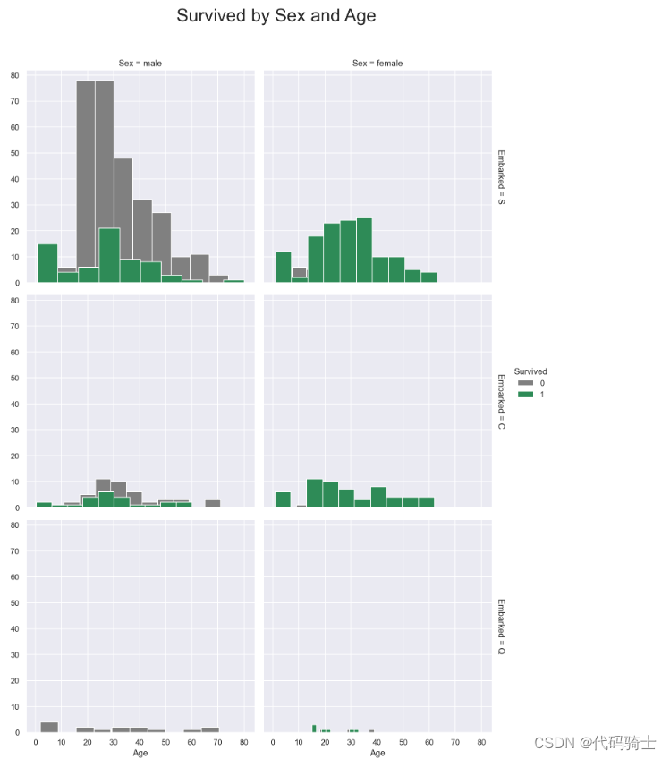
g = sns.FacetGrid(train, size=5,hue="Survived", col ="Sex", margin_titles=True,
                palette=pal,)
g.map(plt.scatter, "Fare", "Age",edgecolor="w").add_legend()
g.fig.suptitle("Survived by Sex, Fare and Age", size = 25)
plt.subplots_adjust(top=0.85)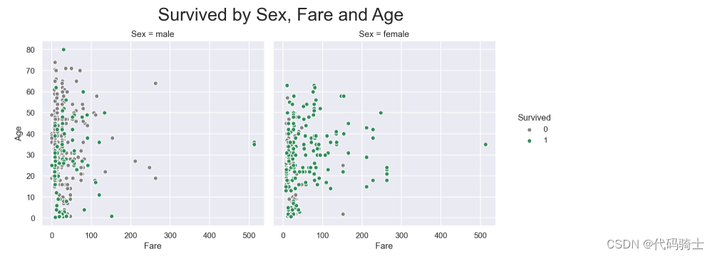
## factor plot
sns.factorplot(x = "Parch", y = "Survived", data = train,kind = "point",size = 8)
plt.title("Factorplot of Parents/Children survived", fontsize = 25)
plt.subplots_adjust(top=1)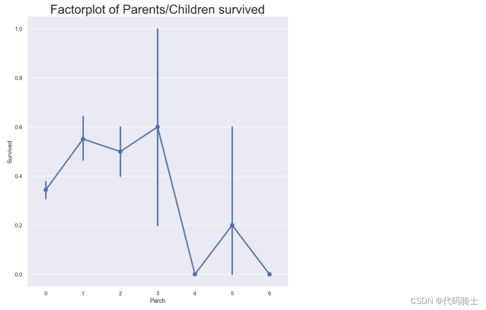
sns.factorplot(x =  "SibSp", y = "Survived", data = train,kind = "point",size = 8)
plt.title('Factorplot of Sibilings/Spouses survived', fontsize = 25)
plt.subplots_adjust(top=0.85)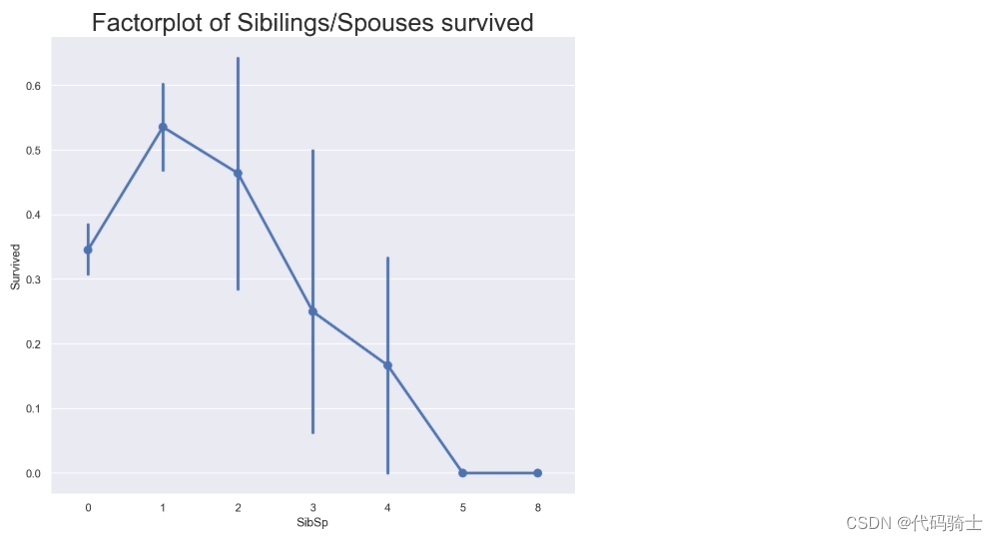
# Placing 0 for female and
# 1 for male in the "Sex" column.
train['Sex'] = train.Sex.apply(lambda x: 0 if x == "female" else 1)
test['Sex'] = test.Sex.apply(lambda x: 0 if x == "female" else 1)
train.describe()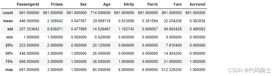
# Overview(Survived vs non survied)
survived_summary = train.groupby("Survived")
survived_summary.mean().reset_index()
survived_summary = train.groupby("Sex")
survived_summary.mean().reset_index()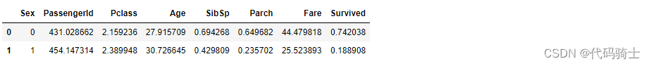
survived_summary = train.groupby("Pclass")
survived_summary.mean().reset_index()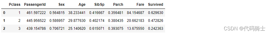
pd.DataFrame(abs(train.corr()['Survived']).sort_values(ascending = False))
## get the most important variables.
corr = train.corr()**2
corr.Survived.sort_values(ascending=False)
## heatmeap to see the correlation between features.
# Generate a mask for the upper triangle (taken from seaborn example gallery)
import numpy as np
mask = np.zeros_like(train.corr(), dtype=np.bool)
mask[np.triu_indices_from(mask)] = True
sns.set_style('whitegrid')
plt.subplots(figsize = (15,12))
sns.heatmap(train.corr(),
            annot=True,
            mask = mask,
            cmap = 'RdBu', ## in order to reverse the bar replace "RdBu" with "RdBu_r"
            linewidths=.9,
            linecolor='white',
            fmt='.2g',
            center = 0,
            square=True)
plt.title("Correlations Among Features", y = 1.03,fontsize = 20, pad = 40);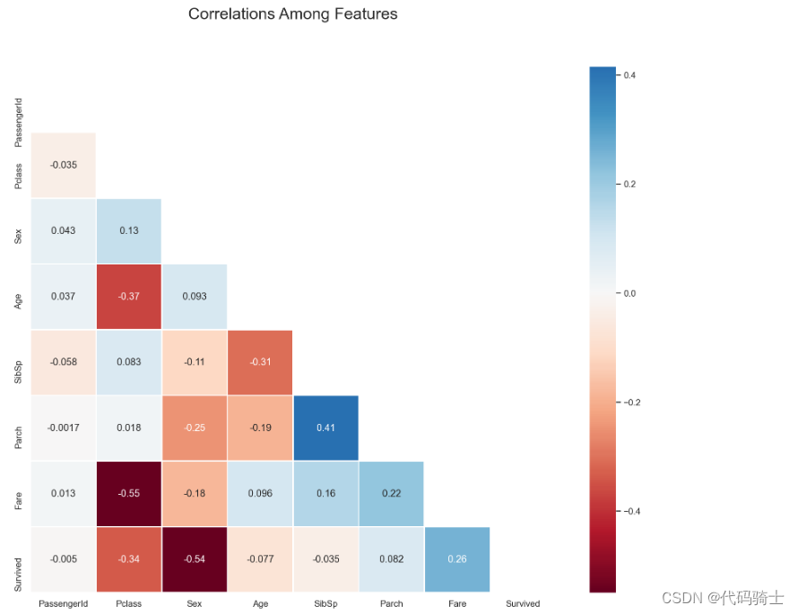
male_mean = train[train['Sex'] == 1].Survived.mean()

female_mean = train[train['Sex'] == 0].Survived.mean()
print ("Male survival mean: " + str(male_mean))
print ("female survival mean: " + str(female_mean))

print ("The mean difference between male and female survival rate: " + str(female_mean - male_mean))
Male survival mean: 0.18890814558058924 female survival mean: 0.7420382165605095 The mean difference between male and female survival rate: 0.5531300709799203
# separating male and female dataframe.
import random
male = train[train['Sex'] == 1]
female = train[train['Sex'] == 0]

## empty list for storing mean sample
m_mean_samples = []
f_mean_samples = []

for i in range(50):
    m_mean_samples.append(np.mean(random.sample(list(male['Survived']),50,)))
    f_mean_samples.append(np.mean(random.sample(list(female['Survived']),50,)))


# Print them out
print (f"Male mean sample mean: {round(np.mean(m_mean_samples),2)}")
print (f"Female mean sample mean: {round(np.mean(f_mean_samples),2)}")
print (f"Difference between male and female mean sample mean: {round(np.mean(f_mean_samples) - np.mean(m_mean_samples),2)}")
Male mean sample mean: 0.18 Female mean sample mean: 0.74 Difference between male and female mean sample mean: 0.56
train.Name0 Braund, Mr. Owen Harris
1 Cumings, Mrs. John Bradley (Florence Briggs Th...
2 Heikkinen, Miss. Laina
3 Futrelle, Mrs. Jacques Heath (Lily May Peel)
4 Allen, Mr. William Henry
...
886 Montvila, Rev. Juozas
887 Graham, Miss. Margaret Edith
888 Johnston, Miss. Catherine Helen "Carrie"
889 Behr, Mr. Karl Howell
890 Dooley, Mr. Patrick
Name: Name, Length: 891, dtype: object
# Creating a new colomn with a
train['name_length'] = [len(i) for i in train.Name]
test['name_length'] = [len(i) for i in test.Name]

def name_length_group(size):
    a = ''
    if (size <=20):
        a = 'short'
    elif (size <=35):
        a = 'medium'
    elif (size <=45):
        a = 'good'
    else:
        a = 'long'
    return a


train['nLength_group'] = train['name_length'].map(name_length_group)
test['nLength_group'] = test['name_length'].map(name_length_group)

## Here "map" is python's built-in function.
## "map" function basically takes a function and
## returns an iterable list/tuple or in this case series.
## However,"map" can also be used like map(function) e.g. map(name_length_group)
## or map(function, iterable{list, tuple}) e.g. map(name_length_group, train[feature]]).
## However, here we don't need to use parameter("size") for name_length_group because when we
## used the map function like ".map" with a series before dot, we are basically hinting that series
## and the iterable. This is similar to .append approach in python. list.append(a) meaning applying append on list.


## cuts the column by given bins based on the range of name_length
#group_names = ['short', 'medium', 'good', 'long']
#train['name_len_group'] = pd.cut(train['name_length'], bins = 4, labels=group_names)
## get the title from the name
train["title"] = [i.split('.')[0] for i in train.Name]
train["title"] = [i.split(',')[1] for i in train.title]
## Whenever we split like that, there is a good change that
#we will end up with white space around our string values. Let's check that.print(train.title.unique())[' Mr' ' Mrs' ' Miss' ' Master' ' Don' ' Rev' ' Dr' ' Mme' ' Ms' ' Major' ' Lady' ' Sir' ' Mlle' ' Col' ' Capt' ' the Countess' ' Jonkheer']
## Let's fix that
train.title = train.title.apply(lambda x: x.strip())
## We can also combile all three lines above for test set here
test['title'] = [i.split('.')[0].split(',')[1].strip() for i in test.Name]
## However it is important to be able to write readable code, and the line above is not so readable. ## Let's replace some of the rare values with the keyword 'rare' and other word choice of our own.
## train Data
train["title"] = [i.replace('Ms', 'Miss') for i in train.title]
train["title"] = [i.replace('Mlle', 'Miss') for i in train.title]
train["title"] = [i.replace('Mme', 'Mrs') for i in train.title]
train["title"] = [i.replace('Dr', 'rare') for i in train.title]
train["title"] = [i.replace('Col', 'rare') for i in train.title]
train["title"] = [i.replace('Major', 'rare') for i in train.title]
train["title"] = [i.replace('Don', 'rare') for i in train.title]
train["title"] = [i.replace('Jonkheer', 'rare') for i in train.title]
train["title"] = [i.replace('Sir', 'rare') for i in train.title]
train["title"] = [i.replace('Lady', 'rare') for i in train.title]
train["title"] = [i.replace('Capt', 'rare') for i in train.title]
train["title"] = [i.replace('the Countess', 'rare') for i in train.title]
train["title"] = [i.replace('Rev', 'rare') for i in train.title]
## Now in programming there is a term called DRY(Don't repeat yourself), whenever we are repeating
## same code over and over again, there should be a light-bulb turning on in our head and make us think
## to code in a way that is not repeating or dull. Let's write a function to do exactly what we
## did in the code above, only not repeating and more interesting.## we are writing a function that can help us modify title column
def fuse_title(feature):
"""
This function helps modifying the title column
"""
result = ''
if feature in ['the Countess','Capt','Lady','Sir','Jonkheer','Don','Major','Col', 'Rev', 'Dona', 'Dr']:
result = 'rare'
elif feature in ['Ms', 'Mlle']:
result = 'Miss'
elif feature == 'Mme':
result = 'Mrs'
else:
result = feature
return result
test.title = test.title.map(fuse_title)
train.title = train.title.map(fuse_title)print(train.title.unique())
print(test.title.unique())['Mr' 'Mrs' 'Miss' 'Master' 'rare'] ['Mr' 'Mrs' 'Miss' 'Master' 'rare']
## Family_size seems like a good feature to create
train['family_size'] = train.SibSp + train.Parch+1
test['family_size'] = test.SibSp + test.Parch+1
## bin the family size.
def family_group(size):
"""
This funciton groups(loner, small, large) family based on family size
"""
a = ''
if (size <= 1):
a = 'loner'
elif (size <= 4):
a = 'small'
else:
a = 'large'
return a## apply the family_group function in family_size
train['family_group'] = train['family_size'].map(family_group)
test['family_group'] = test['family_size'].map(family_group)train['is_alone'] = [1 if i<2 else 0 for i in train.family_size]
test['is_alone'] = [1 if i<2 else 0 for i in test.family_size]#train.Ticket.value_counts().sample(10)
train.Ticket.value_counts()CA. 2343 7
347082 7
1601 7
3101295 6
347088 6
..
12460 1
STON/O2. 3101282 1
349242 1
A/5 21172 1
A/5. 851 1
Name: Ticket, Length: 681, dtype: int64
train.drop(['Ticket'], axis=1, inplace=True)

test.drop(['Ticket'], axis=1, inplace=True)
## Calculating fare based on family size.
train['calculated_fare'] = train.Fare/train.family_size
test['calculated_fare'] = test.Fare/test.family_sizedef fare_group(fare):
"""
This function creates a fare group based on the fare provided
"""
a= ''
if fare <= 4:
a = 'Very_low'
elif fare <= 10:
a = 'low'
elif fare <= 20:
a = 'mid'
elif fare <= 45:
a = 'high'
else:
a = "very_high"
return a
train['fare_group'] = train['calculated_fare'].map(fare_group)
test['fare_group'] = test['calculated_fare'].map(fare_group)
#train['fare_group'] = pd.cut(train['calculated_fare'], bins = 4, labels=groups)train['fare_group']0 Very_low
1 high
2 low
3 high
4 low
...
886 mid
887 high
888 low
889 high
890 low
Name: fare_group, Length: 891, dtype: object
train.drop(['PassengerId'], axis=1, inplace=True)

test.drop(['PassengerId'], axis=1, inplace=True)
train = pd.get_dummies(train, columns=['title',"Pclass", 'Cabin','Embarked','nLength_group', 'family_group', 'fare_group'], drop_first=False)
test = pd.get_dummies(test, columns=['title',"Pclass",'Cabin','Embarked','nLength_group', 'family_group', 'fare_group'], drop_first=False)
train.drop(['family_size','Name', 'Fare','name_length'], axis=1, inplace=True)
test.drop(['Name','family_size',"Fare",'name_length'], axis=1, inplace=True)
## rearranging the columns so that I can easily use the dataframe to predict the missing age values.
train = pd.concat([train[["Survived", "Age", "Sex","SibSp","Parch"]], train.loc[:,"is_alone":]], axis=1)
test = pd.concat([test[["Age", "Sex"]], test.loc[:,"SibSp":]], axis=1)
RandomForestRegressor预测年龄
## Importing RandomForestRegressor
from sklearn.ensemble import RandomForestRegressor

## writing a function that takes a dataframe with missing values and outputs it by filling the missing values.
def completing_age(df):
    ## gettting all the features except survived
    age_df = df.loc[:,"Age":]

    temp_train = age_df.loc[age_df.Age.notnull()] ## df with age values
    temp_test = age_df.loc[age_df.Age.isnull()] ## df without age values

    y = temp_train.Age.values ## setting target variables(age) in y
    x = temp_train.loc[:, "Sex":].values

    rfr = RandomForestRegressor(n_estimators=1500, n_jobs=-1)
    rfr.fit(x, y)

    predicted_age = rfr.predict(temp_test.loc[:, "Sex":])

    df.loc[df.Age.isnull(), "Age"] = predicted_age


    return df

## Implementing the completing_age function in both train and test dataset.
completing_age(train)
completing_age(test);
## Let's look at the his
plt.subplots(figsize = (22,10),)
sns.distplot(train.Age, bins = 100, kde = True, rug = False, norm_hist=False);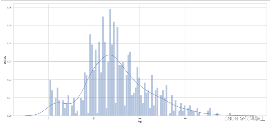
## create bins for age
def age_group_fun(age):
    """
    This function creates a bin for age
    """
    a = ''
    if age <= 1:
        a = 'infant'
    elif age <= 4:
        a = 'toddler'
    elif age <= 13:
        a = 'child'
    elif age <= 18:
        a = 'teenager'
    elif age <= 35:
        a = 'Young_Adult'
    elif age <= 45:
        a = 'adult'
    elif age <= 55:
        a = 'middle_aged'
    elif age <= 65:
        a = 'senior_citizen'
    else:
        a = 'old'
    return a

## Applying "age_group_fun" function to the "Age" column.
train['age_group'] = train['Age'].map(age_group_fun)
test['age_group'] = test['Age'].map(age_group_fun)

## Creating dummies for "age_group" feature.
train = pd.get_dummies(train,columns=['age_group'], drop_first=True)
test = pd.get_dummies(test,columns=['age_group'], drop_first=True);
# separating our independent and dependent variable
X = train.drop(['Survived'], axis = 1)
y = train["Survived"]from sklearn.model_selection import train_test_split
X_train, X_test, y_train, y_test = train_test_split(X, y,test_size = .33, random_state=0)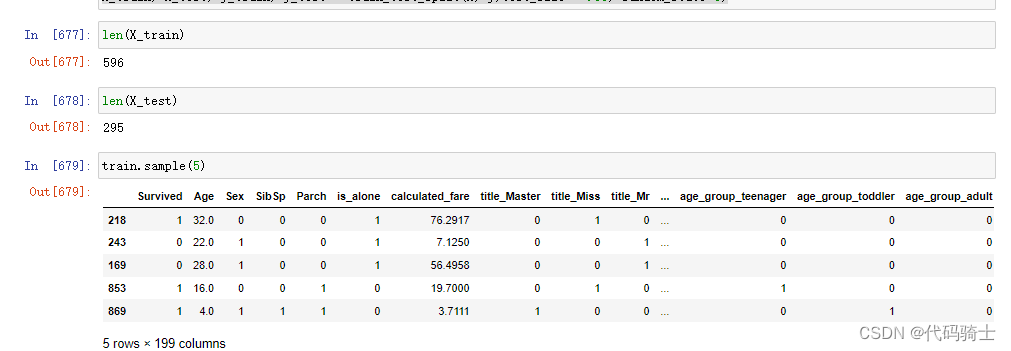
## getting the headers
headers = X_train.columns
X_train.head()
# Feature Scaling
## We will be using standardscaler to transform
from sklearn.preprocessing import StandardScaler
std_scale = StandardScaler()

## transforming "train_x"
X_train = std_scale.fit_transform(X_train)
## transforming "test_x"
X_test = std_scale.transform(X_test)

## transforming "The testset"
#test = st_scale.transform(test)
pd.DataFrame(X_train, columns=headers).head()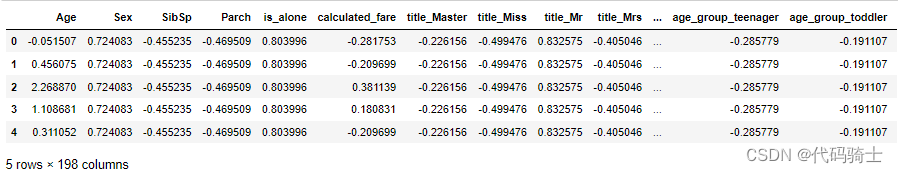
LogisticRegression建模
A regression model that uses L1 regularization technique is called Lasso Regression and model which uses L2 is called Ridge Regression. The key difference between these two is the penalty term. Ridge regression adds “squared magnitude” of coefficient as penalty term to the loss function
# import LogisticRegression model in python.
from sklearn.linear_model import LogisticRegression
from sklearn.metrics import mean_absolute_error, accuracy_score

## call on the model object
logreg = LogisticRegression(solver='liblinear',
                            penalty= 'l1',random_state = 42

                            )

## fit the model with "train_x" and "train_y"
logreg.fit(X_train,y_train)

y_pred = logreg.predict(X_test)
from sklearn.metrics import classification_report, confusion_matrix
# printing confision matrix
pd.DataFrame(confusion_matrix(y_test,y_pred),\
            columns=["Predicted Not-Survived", "Predicted Survived"],\
            index=["Not-Survived","Survived"] )
from sklearn.metrics import confusion_matrix
from sklearn.metrics import ConfusionMatrixDisplay

y_pred = logreg.predict(X_test)
cm = confusion_matrix(y_test, y_pred)

cm_display = ConfusionMatrixDisplay(cm,display_labels='').plot() 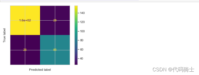
from sklearn.metrics import accuracy_score
accuracy_score(y_test, y_pred)
0.8305084745762712
from sklearn.metrics import recall_score
recall_score(y_test, y_pred)
0.7927927927927928
from sklearn.metrics import precision_score
precision_score(y_test, y_pred)
0.7652173913043478
from sklearn.metrics import classification_report, balanced_accuracy_score
print(classification_report(y_test, y_pred))
precision recall f1-score support
0 0.87 0.85 0.86 184
1 0.77 0.79 0.78 111
accuracy 0.83 295
macro avg 0.82 0.82 0.82 295
weighted avg 0.83 0.83 0.83 295
from sklearn.metrics import roc_curve, auc
#plt.style.use('seaborn-pastel')
y_score = logreg.decision_function(X_test)

FPR, TPR, _ = roc_curve(y_test, y_score)
ROC_AUC = auc(FPR, TPR)
print (ROC_AUC)

plt.figure(figsize =[11,9])
plt.plot(FPR, TPR, label= 'ROC curve(area = %0.2f)'%ROC_AUC, linewidth= 4)
plt.plot([0,1],[0,1], 'k--', linewidth = 4)
plt.xlim([0.0,1.0])
plt.ylim([0.0,1.05])
plt.xlabel('False Positive Rate', fontsize = 18)
plt.ylabel('True Positive Rate', fontsize = 18)
plt.title('ROC for Titanic survivors', fontsize= 18)
plt.show()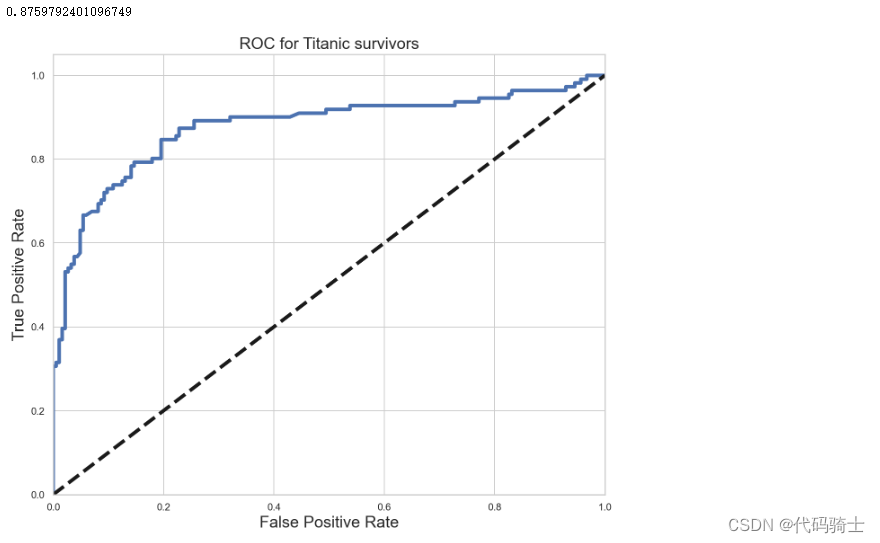
from sklearn.metrics import precision_recall_curve

y_score = logreg.decision_function(X_test)

precision, recall, _ = precision_recall_curve(y_test, y_score)
PR_AUC = auc(recall, precision)

plt.figure(figsize=[11,9])
plt.plot(recall, precision, label='PR curve (area = %0.2f)' % PR_AUC, linewidth=4)
plt.xlabel('Recall', fontsize=18)
plt.ylabel('Precision', fontsize=18)
plt.title('Precision Recall Curve for Titanic survivors', fontsize=18)
plt.legend(loc="lower right")
plt.show()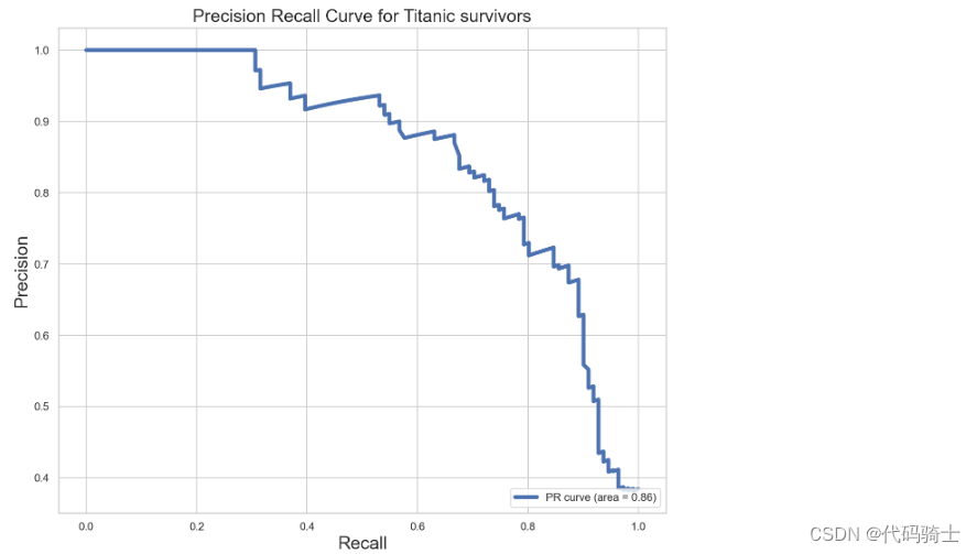
引入GridSearchCV
GridSearch stands for the fact that we are searching for optimal parameter/parameters over a "grid." These optimal parameters are also known as Hyperparameters. The Hyperparameters are model parameters that are set before fitting the model and determine the behavior of the model.
from sklearn.model_selection import GridSearchCV
from sklearn.model_selection import StratifiedShuffleSplit
# C_vals is the alpla value of lasso and ridge regression(as
# alpha increases the model complexity decreases,)

## remember effective alpha scores are 0<alpha<infinity
C_vals = [0.2,0.3,0.4,0.5,0.6,0.7,0.8,0.9,1]

## Choose a cross validation strategy.
cv = StratifiedShuffleSplit(n_splits = 10, test_size = .25)

## setting param for param_grid in GridSearchCV.
param = {'C': C_vals}

logreg = LogisticRegression()
## Calling on GridSearchCV object.
grid = GridSearchCV(
    estimator=LogisticRegression(),
    param_grid = param,
    scoring = 'accuracy',
    n_jobs =-1,
    cv = cv
)
## Fitting the model
grid.fit(X, y)
GridSearchCV(cv=StratifiedShuffleSplit(n_splits=10, random_state=None, test_size=0.25,
train_size=None),
error_score=nan,
estimator=LogisticRegression(C=1.0, class_weight=None, dual=False,
fit_intercept=True,
intercept_scaling=1, l1_ratio=None,
max_iter=100, multi_class='auto',
n_jobs=None, penalty='l2',
random_state=None, solver='lbfgs',
tol=0.0001, verbose=0,
warm_start=False),
iid='deprecated', n_jobs=-1,
param_grid={'C': [0.2, 0.3, 0.4, 0.5, 0.6, 0.7, 0.8, 0.9, 1]},
pre_dispatch='2*n_jobs', refit=True, return_train_score=False,
scoring='accuracy', verbose=0)
## Getting the best of everything.
print (grid.best_score_)
print (grid.best_params_)
print(grid.best_estimator_)
0.8251121076233184
{'C': 0.9}
LogisticRegression(C=0.9, class_weight=None, dual=False, fit_intercept=True,
intercept_scaling=1, l1_ratio=None, max_iter=100,
multi_class='auto', n_jobs=None, penalty='l2',
random_state=None, solver='lbfgs', tol=0.0001, verbose=0,
warm_start=False)
### Using the best parameters from the grid-search.
logreg_grid = grid.best_estimator_
logreg_grid.score(X,y)
引入RandomizedSearchCV
Randomized search is a close cousin of grid search. It doesn't always provide the best result but its fast.
from sklearn.model_selection import RandomizedSearchCV

rand1 = RandomizedSearchCV(
    estimator=LogisticRegression(),
    param_distributions = param,
    scoring = 'accuracy',
    n_jobs =-1,
    cv = cv
)
## Fitting the model
rand1.fit(X, y)
RandomizedSearchCV(cv=StratifiedShuffleSplit(n_splits=10, random_state=None, test_size=0.25,
train_size=None),
error_score=nan,
estimator=LogisticRegression(C=1.0, class_weight=None,
dual=False, fit_intercept=True,
intercept_scaling=1,
l1_ratio=None, max_iter=100,
multi_class='auto', n_jobs=None,
penalty='l2', random_state=None,
solver='lbfgs', tol=0.0001,
verbose=0, warm_start=False),
iid='deprecated', n_iter=10, n_jobs=-1,
param_distributions={'C': [0.2, 0.3, 0.4, 0.5, 0.6, 0.7, 0.8,
0.9, 1]},
pre_dispatch='2*n_jobs', random_state=None, refit=True,
return_train_score=False, scoring='accuracy', verbose=0)
## Getting the best of everything.
print (rand1.best_score_)
print (rand1.best_params_)
print(rand1.best_estimator_)
0.8210762331838565
{'C': 0.4}
LogisticRegression(C=0.4, class_weight=None, dual=False, fit_intercept=True,
intercept_scaling=1, l1_ratio=None, max_iter=100,
multi_class='auto', n_jobs=None, penalty='l2',
random_state=None, solver='lbfgs', tol=0.0001, verbose=0,
warm_start=False)
logreg_rand = rand1.best_estimator_
logreg_rand.score(X,y)
0.8361391694725028
Decision Tree建模
from sklearn.tree import DecisionTreeClassifier
max_depth = range(1,30)
max_feature = [21,22,23,24,25,26,28,29,30,'auto']
criterion=["entropy", "gini"]

param = {'max_depth':max_depth,
         'max_features':max_feature,
         'criterion': criterion}
grid = GridSearchCV(DecisionTreeClassifier(),
                                param_grid = param,
                                 verbose=False,
                                 cv=StratifiedShuffleSplit(n_splits=20, random_state=15),
                                n_jobs = -1)
grid.fit(X, y)
GridSearchCV(cv=StratifiedShuffleSplit(n_splits=20, random_state=15, test_size=None,
train_size=None),
error_score=nan,
estimator=DecisionTreeClassifier(ccp_alpha=0.0, class_weight=None,
criterion='gini', max_depth=None,
max_features=None,
max_leaf_nodes=None,
min_impurity_decrease=0.0,
min_impurity_split=None,
min_samples_leaf=1,
min_samples_split=2,
min_weight_fraction_leaf=0.0,
presort='deprecated',
random_state=None,
splitter='best'),
iid='deprecated', n_jobs=-1,
param_grid={'criterion': ['entropy', 'gini'],
'max_depth': range(1, 30),
'max_features': [21, 22, 23, 24, 25, 26, 28, 29, 30,
'auto']},
pre_dispatch='2*n_jobs', refit=True, return_train_score=False,
scoring=None, verbose=False)
print( grid.best_params_)
print (grid.best_score_)
print (grid.best_estimator_)
{'criterion': 'gini', 'max_depth': 8, 'max_features': 26}
0.8211111111111112
DecisionTreeClassifier(ccp_alpha=0.0, class_weight=None, criterion='gini',
max_depth=8, max_features=26, max_leaf_nodes=None,
min_impurity_decrease=0.0, min_impurity_split=None,
min_samples_leaf=1, min_samples_split=2,
min_weight_fraction_leaf=0.0, presort='deprecated',
random_state=None, splitter='best')
dectree_grid = grid.best_estimator_
## using the best found hyper paremeters to get the score.
dectree_grid.score(X,y)
0.8574635241301908
RandomForest建模
from sklearn.model_selection import GridSearchCV, StratifiedKFold, StratifiedShuffleSplit
from sklearn.ensemble import RandomForestClassifier
n_estimators = [140,145,150,155,160];
max_depth = range(1,10);
criterions = ['gini', 'entropy'];
cv = StratifiedShuffleSplit(n_splits=10, test_size=.30, random_state=15)


parameters = {'n_estimators':n_estimators,
              'max_depth':max_depth,
              'criterion': criterions

        }
grid = GridSearchCV(estimator=RandomForestClassifier(max_features='auto'),
                                 param_grid=parameters,
                                 cv=cv,
                                 n_jobs = -1)
grid.fit(X,y)
GridSearchCV(cv=StratifiedShuffleSplit(n_splits=10, random_state=15, test_size=0.3,
train_size=None),
error_score=nan,
estimator=RandomForestClassifier(bootstrap=True, ccp_alpha=0.0,
class_weight=None,
criterion='gini', max_depth=None,
max_features='auto',
max_leaf_nodes=None,
max_samples=None,
min_impurity_decrease=0.0,
min_impurity_split=None,
min_samples_leaf=1,
min_samples_split=2,
min_weight_fraction_leaf=0.0,
n_estimators=100, n_jobs=None,
oob_score=False,
random_state=None, verbose=0,
warm_start=False),
iid='deprecated', n_jobs=-1,
param_grid={'criterion': ['gini', 'entropy'],
'max_depth': range(1, 10),
'n_estimators': [140, 145, 150, 155, 160]},
pre_dispatch='2*n_jobs', refit=True, return_train_score=False,
scoring=None, verbose=0)print (grid.best_score_)
print (grid.best_params_)
print (grid.best_estimator_)0.835820895522388
{'criterion': 'entropy', 'max_depth': 6, 'n_estimators': 150}
RandomForestClassifier(bootstrap=True, ccp_alpha=0.0, class_weight=None,
criterion='entropy', max_depth=6, max_features='auto',
max_leaf_nodes=None, max_samples=None,
min_impurity_decrease=0.0, min_impurity_split=None,
min_samples_leaf=1, min_samples_split=2,
min_weight_fraction_leaf=0.0, n_estimators=150,
n_jobs=None, oob_score=False, random_state=None,
verbose=0, warm_start=False)
rf_grid = grid.best_estimator_
rf_grid.score(X,y)0.8574635241301908
Feature Importance
column_names = X1.columns
feature_importances = pd.DataFrame(rf_grid.feature_importances_,
index = column_names,
columns=['importance'])
feature_importances.sort_values(by='importance', ascending=False).head(15)
AdaBoost建模
from sklearn.ensemble import AdaBoostClassifier
adaBoost = AdaBoostClassifier(base_estimator=None,
learning_rate=1.0,
n_estimators=100)
adaBoost.fit(X_train, y_train)
y_pred = adaBoost.predict(X_test)
from sklearn.metrics import accuracy_score
accuracy_score(y_test, y_pred)0.8033898305084746
from sklearn.model_selection import GridSearchCV
from sklearn.model_selection import StratifiedShuffleSplit
n_estimators = [80,100,140,145,150,160, 170,175,180,185];
cv = StratifiedShuffleSplit(n_splits=10, test_size=.30, random_state=15)
learning_r = [0.1,1,0.01,0.5]
parameters = {'n_estimators':n_estimators,
'learning_rate':learning_r
}
grid = GridSearchCV(AdaBoostClassifier(base_estimator= None, ## If None, then the base estimator is a decision tree.
),
param_grid=parameters,
cv=cv,
n_jobs = -1)
grid.fit(X,y) GridSearchCV(cv=StratifiedShuffleSplit(n_splits=10, random_state=15, test_size=0.3,
train_size=None),
error_score=nan,
estimator=AdaBoostClassifier(algorithm='SAMME.R',
base_estimator=None,
learning_rate=1.0, n_estimators=50,
random_state=None),
iid='deprecated', n_jobs=-1,
param_grid={'learning_rate': [0.1, 1, 0.01, 0.5],
'n_estimators': [80, 100, 140, 145, 150, 160, 170, 175,
180, 185]},
pre_dispatch='2*n_jobs', refit=True, return_train_score=False,
scoring=None, verbose=0)
## Getting the best of everything.
print (grid.best_score_)
print (grid.best_params_)
print(grid.best_estimator_)0.825
{'learning_rate': 0.1, 'n_estimators': 80}
AdaBoostClassifier(algorithm='SAMME.R', base_estimator=None, learning_rate=0.1,
n_estimators=80, random_state=None)
ada_grid = grid.best_estimator_
ada_grid.score(X,y)0.8316498316498316
Gradient Boosting梯度提升建模
# Gradient Boosting Classifier
from sklearn.ensemble import GradientBoostingClassifier
gradient_boost = GradientBoostingClassifier()
gradient_boost.fit(X_train, y_train)
y_pred = gradient_boost.predict(X_test)
gradient_accy = round(accuracy_score(y_pred, y_test), 3)
print(gradient_accy)0.817
grid = GridSearchCV(GradientBoostingClassifier(),
param_grid=parameters,
cv=cv,
n_jobs = -1)
grid.fit(X,y) GridSearchCV(cv=StratifiedShuffleSplit(n_splits=10, random_state=15, test_size=0.3,
train_size=None),
error_score=nan,
estimator=GradientBoostingClassifier(ccp_alpha=0.0,
criterion='friedman_mse',
init=None, learning_rate=0.1,
loss='deviance', max_depth=3,
max_features=None,
max_leaf_nodes=None,
min_impurity_decrease=0.0,
min_impurity_split=None,
min_samples_leaf...
n_iter_no_change=None,
presort='deprecated',
random_state=None,
subsample=1.0, tol=0.0001,
validation_fraction=0.1,
verbose=0, warm_start=False),
iid='deprecated', n_jobs=-1,
param_grid={'learning_rate': [0.1, 1, 0.01, 0.5],
'n_estimators': [80, 100, 140, 145, 150, 160, 170, 175,
180, 185]},
pre_dispatch='2*n_jobs', refit=True, return_train_score=False,
scoring=None, verbose=0)
## Getting the best of everything.
print (grid.best_score_)
print (grid.best_params_)
print(grid.best_estimator_)0.8376865671641791
{'learning_rate': 0.01, 'n_estimators': 140}
GradientBoostingClassifier(ccp_alpha=0.0, criterion='friedman_mse', init=None,
learning_rate=0.01, loss='deviance', max_depth=3,
max_features=None, max_leaf_nodes=None,
min_impurity_decrease=0.0, min_impurity_split=None,
min_samples_leaf=1, min_samples_split=2,
min_weight_fraction_leaf=0.0, n_estimators=140,
n_iter_no_change=None, presort='deprecated',
random_state=None, subsample=1.0, tol=0.0001,
validation_fraction=0.1, verbose=0,
warm_start=False)
gb_grid = grid.best_estimator_
gb_grid.score(X,y)0.8406285072951739
Support Vector Machine建模
from sklearn.svm import SVC
Cs = [0.001, 0.01, 0.1, 1,1.5,2,2.5,3,4,5, 10] ## penalty parameter C for the error term.
gammas = [0.0001,0.001, 0.01, 0.1, 1]
param_grid = {'C': Cs, 'gamma' : gammas}
cv = StratifiedShuffleSplit(n_splits=10, test_size=.30, random_state=15)
grid_search = GridSearchCV(SVC(kernel = 'rbf', probability=True), param_grid, cv=cv) ## 'rbf' stands for gaussian kernel
grid_search.fit(X,y)GridSearchCV(cv=StratifiedShuffleSplit(n_splits=10, random_state=15, test_size=0.3,
train_size=None),
error_score=nan,
estimator=SVC(C=1.0, break_ties=False, cache_size=200,
class_weight=None, coef0=0.0,
decision_function_shape='ovr', degree=3,
gamma='scale', kernel='rbf', max_iter=-1,
probability=True, random_state=None, shrinking=True,
tol=0.001, verbose=False),
iid='deprecated', n_jobs=None,
param_grid={'C': [0.001, 0.01, 0.1, 1, 1.5, 2, 2.5, 3, 4, 5, 10],
'gamma': [0.0001, 0.001, 0.01, 0.1, 1]},
pre_dispatch='2*n_jobs', refit=True, return_train_score=False,
scoring=None, verbose=0)
print(grid_search.best_score_)
print(grid_search.best_params_)
print(grid_search.best_estimator_)0.835820895522388
{'C': 1, 'gamma': 0.01}
SVC(C=1, break_ties=False, cache_size=200, class_weight=None, coef0=0.0,
decision_function_shape='ovr', degree=3, gamma=0.01, kernel='rbf',
max_iter=-1, probability=True, random_state=None, shrinking=True, tol=0.001,
verbose=False)
# using the best found hyper paremeters to get the score.
svm_grid = grid_search.best_estimator_
svm_grid.score(X,y)0.8372615039281706
svm_grid.predict(X_test)array([0, 0, 0, 1, 1, 0, 1, 1, 0, 1, 0, 1, 0, 1, 1, 1, 0, 0, 0, 1, 0, 1,
0, 0, 1, 1, 0, 1, 1, 0, 0, 1, 0, 0, 0, 0, 0, 0, 0, 0, 0, 0, 0, 0,
1, 0, 0, 1, 0, 0, 0, 0, 1, 0, 0, 0, 0, 0, 0, 0, 0, 0, 1, 0, 1, 0,
1, 0, 1, 1, 1, 0, 0, 0, 0, 1, 0, 0, 0, 0, 0, 1, 1, 0, 0, 1, 1, 1,
1, 0, 0, 0, 1, 1, 0, 0, 1, 0, 0, 0, 0, 0, 0, 0, 1, 1, 1, 0, 0, 1,
0, 1, 0, 1, 0, 1, 1, 1, 0, 1, 0, 0, 0, 0, 0, 0, 0, 0, 0, 0, 1, 0,
0, 1, 0, 0, 0, 1, 0, 0, 0, 1, 0, 1, 1, 1, 0, 1, 1, 0, 0, 1, 1, 0,
1, 0, 1, 0, 1, 1, 0, 0, 1, 1, 0, 0, 0, 0, 0, 0, 0, 1, 0, 0, 1, 0,
1, 0, 0, 1, 0, 0, 0, 0, 0, 0, 1, 0, 0, 1, 1, 0, 1, 1, 0, 0, 0, 1,
0, 0, 0, 1, 0, 1, 0, 0, 1, 0, 1, 0, 0, 0, 0, 1, 0, 0, 0, 1, 0, 1,
0, 1, 1, 0, 0, 0, 0, 1, 0, 0, 0, 1, 1, 1, 0, 0, 1, 1, 1, 0, 0, 1,
0, 0, 1, 1, 1, 0, 0, 1, 0, 0, 0, 0, 0, 1, 1, 0, 0, 0, 0, 0, 0, 0,
0, 0, 1, 0, 0, 1, 0, 0, 1, 1, 0, 0, 0, 0, 1, 1, 0, 1, 0, 1, 0, 0,
0, 0, 0, 0, 0, 0, 1, 1, 1], dtype=int64)
Xgboost建模
from xgboost import XGBClassifier
XGBC = XGBClassifier()
XGBC.fit(X_train, y_train)
y_pred = XGBC.predict(X_test)
XGBC_accy = round(accuracy_score(y_pred, y_test), 3)
print(XGBC_accy)0.841
grid = GridSearchCV(XGBClassifier(base_estimator= 100,
),
param_grid=parameters,
cv=cv,
n_jobs = -1)
grid.fit(X,y) GridSearchCV(cv=StratifiedShuffleSplit(n_splits=10, random_state=15, test_size=0.3,
train_size=None),
error_score=nan,
estimator=XGBClassifier(base_estimator=100, base_score=0.5,
booster='gbtree', colsample_bylevel=1,
colsample_bynode=1, colsample_bytree=1,
gamma=0, learning_rate=0.1,
max_delta_step=0, max_depth=3,
min_child_weight=1, missing=None,
n_estimators=100...one,
objective='binary:logistic',
random_state=0, reg_alpha=0, reg_lambda=1,
scale_pos_weight=1, seed=None, silent=None,
subsample=1, verbosity=1),
iid='deprecated', n_jobs=-1,
param_grid={'learning_rate': [0.1, 1, 0.01, 0.5],
'n_estimators': [80, 100, 140, 145, 150, 160, 170, 175,
180, 185]},
pre_dispatch='2*n_jobs', refit=True, return_train_score=False,
scoring=None, verbose=0)
## Getting the best of everything.
print (grid.best_score_)
print (grid.best_params_)
print(grid.best_estimator_)0.8402985074626865
{'learning_rate': 0.01, 'n_estimators': 140}
XGBClassifier(base_estimator=100, base_score=0.5, booster='gbtree',
colsample_bylevel=1, colsample_bynode=1, colsample_bytree=1,
gamma=0, learning_rate=0.01, max_delta_step=0, max_depth=3,
min_child_weight=1, missing=None, n_estimators=140, n_jobs=1,
nthread=None, objective='binary:logistic', random_state=0,
reg_alpha=0, reg_lambda=1, scale_pos_weight=1, seed=None,
silent=None, subsample=1, verbosity=1)
xgb_grid = grid.best_estimator_
xgb_grid.score(X,y)0.8428731762065096
Bagging Classifier建模
Why use Bagging?
Bagging works best with strong and complex models(for example, fully developed decision trees). However, don't let that fool you to thinking that similar to a decision tree, bagging also overfits the model. Instead, bagging reduces overfitting since a lot of the sample training data are repeated and used to create base estimators. With a lot of equally likely training data, bagging is not very susceptible to overfitting with noisy data, therefore reduces variance. However, the downside is that this leads to an increase in bias.
from sklearn.ensemble import BaggingClassifier
n_estimators = [10,30,50,70,80,150,160, 170,175,180,185];
cv = StratifiedShuffleSplit(n_splits=10, test_size=.30, random_state=15)
parameters = {'n_estimators':n_estimators,}
grid = GridSearchCV(BaggingClassifier(base_estimator= None, ## If None, then the base estimator is a decision tree.
bootstrap_features=False),
param_grid=parameters,
cv=cv,
n_jobs = -1)
grid.fit(X,y) GridSearchCV(cv=StratifiedShuffleSplit(n_splits=10, random_state=15, test_size=0.3,
train_size=None),
error_score=nan,
estimator=BaggingClassifier(base_estimator=None, bootstrap=True,
bootstrap_features=False,
max_features=1.0, max_samples=1.0,
n_estimators=10, n_jobs=None,
oob_score=False, random_state=None,
verbose=0, warm_start=False),
iid='deprecated', n_jobs=-1,
param_grid={'n_estimators': [10, 30, 50, 70, 80, 150, 160, 170,
175, 180, 185]},
pre_dispatch='2*n_jobs', refit=True, return_train_score=False,
scoring=None, verbose=0)
print (grid.best_score_)
print (grid.best_params_)
print (grid.best_estimator_)0.8171641791044777
{'n_estimators': 185}
BaggingClassifier(base_estimator=None, bootstrap=True, bootstrap_features=False,
max_features=1.0, max_samples=1.0, n_estimators=185,
n_jobs=None, oob_score=False, random_state=None, verbose=0,
warm_start=False)
bagging_grid = grid.best_estimator_
bagging_grid.score(X,y)
0.9887766554433222
Extra Trees Classifier建模
from sklearn.ensemble import ExtraTreesClassifier
ExtraTreesClassifier = ExtraTreesClassifier()
ExtraTreesClassifier.fit(X, y)
y_pred = ExtraTreesClassifier.predict(X_test)
extraTree_accy = round(accuracy_score(y_pred, y_test), 3)
print(extraTree_accy)
0.892
K-Nearest Neighbor classifier(KNN)建模 using GridSearchCV
## Importing the model.
from sklearn.neighbors import KNeighborsClassifier
from sklearn.model_selection import cross_val_score
## calling on the model oject.
knn = KNeighborsClassifier(metric='minkowski', p=2)
## knn classifier works by doing euclidian distance


## doing 10 fold staratified-shuffle-split cross validation
cv = StratifiedShuffleSplit(n_splits=10, test_size=.25, random_state=2)

accuracies = cross_val_score(knn, X,y, cv = cv, scoring='accuracy')
print ("Cross-Validation accuracy scores:{}".format(accuracies))
print ("Mean Cross-Validation accuracy score: {}".format(round(accuracies.mean(),3)))
Cross-Validation accuracy scores:[0.78475336 0.76681614 0.79820628 0.81165919 0.81165919 0.79372197 0.77578475 0.8161435 0.78026906 0.8161435 ] Mean Cross-Validation accuracy score: 0.796
## Search for an optimal value of k for KNN.
k_range = range(1,31)
k_scores = []
for k in k_range:
    knn = KNeighborsClassifier(n_neighbors=k)
    scores = cross_val_score(knn, X,y, cv = cv, scoring = 'accuracy')
    k_scores.append(scores.mean())
print("Accuracy scores are: {}\n".format(k_scores))
print ("Mean accuracy score: {}".format(np.mean(k_scores)))
Accuracy scores are: [0.742152466367713, 0.7641255605381165, 0.7878923766816144, 0.7923766816143497, 0.7955156950672645, 0.7986547085201794, 0.794170403587444, 0.7914798206278026, 0.7977578475336322, 0.793273542600897, 0.794170403587444, 0.789237668161435, 0.7946188340807174, 0.7887892376681614, 0.7887892376681613, 0.7865470852017937, 0.7887892376681613, 0.788340807174888, 0.795067264573991, 0.7838565022421525, 0.7865470852017937, 0.7820627802690583, 0.7874439461883408, 0.7798206278026906, 0.784304932735426, 0.7690582959641257, 0.775336322869955, 0.7695067264573991, 0.7748878923766817, 0.768609865470852] Mean accuracy score: 0.7844394618834081
from matplotlib import pyplot as plt
plt.plot(k_range, k_scores)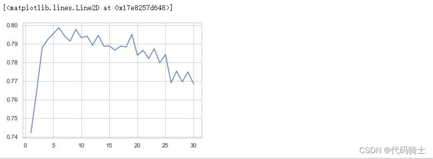
from sklearn.model_selection import GridSearchCV
## trying out multiple values for k
k_range = range(1,31)
##
weights_options=['uniform','distance']
#
param = {'n_neighbors':k_range, 'weights':weights_options}
## Using startifiedShufflesplit.
cv = StratifiedShuffleSplit(n_splits=10, test_size=.30, random_state=15)
# estimator = knn, param_grid = param, n_jobs = -1 to instruct scikit learn to use all available processors.
grid = GridSearchCV(KNeighborsClassifier(), param,cv=cv,verbose = False, n_jobs=-1)
## Fitting the model.
grid.fit(X,y)
GridSearchCV(cv=StratifiedShuffleSplit(n_splits=10, random_state=15, test_size=0.3,
train_size=None),
error_score=nan,
estimator=KNeighborsClassifier(algorithm='auto', leaf_size=30,
metric='minkowski',
metric_params=None, n_jobs=None,
n_neighbors=5, p=2,
weights='uniform'),
iid='deprecated', n_jobs=-1,
param_grid={'n_neighbors': range(1, 31),
'weights': ['uniform', 'distance']},
pre_dispatch='2*n_jobs', refit=True, return_train_score=False,
scoring=None, verbose=False)
print(grid.best_score_)
print(grid.best_params_)
print(grid.best_estimator_)
0.8082089552238806
{'n_neighbors': 8, 'weights': 'uniform'}
KNeighborsClassifier(algorithm='auto', leaf_size=30, metric='minkowski',
metric_params=None, n_jobs=None, n_neighbors=8, p=2,
weights='uniform')
### Using the best parameters from the grid-search.
knn_grid= grid.best_estimator_
knn_grid.score(X,y)
0.8417508417508418
K-Nearest Neighbor classifier(KNN)建模 Using RandomizedSearchCV
from sklearn.model_selection import RandomizedSearchCV
## trying out multiple values for k
k_range = range(1,31)
##
weights_options=['uniform','distance']
#
param = {'n_neighbors':k_range, 'weights':weights_options}
## Using startifiedShufflesplit.
cv = StratifiedShuffleSplit(n_splits=10, test_size=.30)
# estimator = knn, param_grid = param, n_jobs = -1 to instruct scikit learn to use all available processors.
## for RandomizedSearchCV,
grid = RandomizedSearchCV(KNeighborsClassifier(), param,cv=cv,verbose = False, n_jobs=-1, n_iter=40)
## Fitting the model.
grid.fit(X,y)
RandomizedSearchCV(cv=StratifiedShuffleSplit(n_splits=10, random_state=None, test_size=0.3,
train_size=None),
error_score=nan,
estimator=KNeighborsClassifier(algorithm='auto',
leaf_size=30,
metric='minkowski',
metric_params=None,
n_jobs=None, n_neighbors=5,
p=2, weights='uniform'),
iid='deprecated', n_iter=40, n_jobs=-1,
param_distributions={'n_neighbors': range(1, 31),
'weights': ['uniform', 'distance']},
pre_dispatch='2*n_jobs', random_state=None, refit=True,
return_train_score=False, scoring=None, verbose=False)
print (grid.best_score_)
print (grid.best_params_)
print(grid.best_estimator_)
0.8085820895522389
{'weights': 'uniform', 'n_neighbors': 6}
KNeighborsClassifier(algorithm='auto', leaf_size=30, metric='minkowski',
metric_params=None, n_jobs=None, n_neighbors=6, p=2,
weights='uniform')
### Using the best parameters from the grid-search.
knn_ran_grid = grid.best_estimator_
knn_ran_grid.score(X,y)
0.8552188552188552
Gaussian Naive Bayes建模
# Gaussian Naive Bayes
from sklearn.naive_bayes import GaussianNB
from sklearn.metrics import accuracy_score

gaus = GaussianNB()
gaus.fit(X, y)
y_pred = gaus.predict(X_test)
gaus_accy = round(accuracy_score(y_pred, y_test), 3)
print(gaus_accy)
0.81
Gaussian Naive Bayes建模 with Gaussian Process Classifier
from sklearn.gaussian_process import GaussianProcessClassifier
GaussianProcessClassifier = GaussianProcessClassifier()
GaussianProcessClassifier.fit(X, y)
y_pred = GaussianProcessClassifier.predict(X_test)
gau_pro_accy = round(accuracy_score(y_pred, y_test), 3)
print(gau_pro_accy)
VotingClassifier建模
from IPython.display import Image

Image(filename='C:\\Users\\86185\\Desktop\\TempDesktop\\研究内容\\Python学习\\Py机深文字教程+源码\\LessonPythonCode-main\\Lesson26-Voting.png') 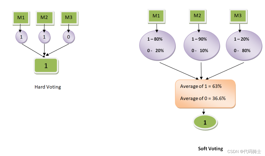
from IPython.display import Image
Image(filename='C:\\Users\\86185\\Desktop\\TempDesktop\\研究内容\\Python学习\\Py机深文字教程+源码\\LessonPythonCode-main\\Lesson26-Voting1.png')
from sklearn.ensemble import VotingClassifier

voting_classifier = VotingClassifier(estimators=[
    ('lr_grid', logreg_grid),
    ('lr_grid1', logreg_rand),
    ('svc', svm_grid),
    ('random_forest', rf_grid),
    ('gradient_boosting',gb_grid),
    ('decision_tree_grid',dectree_grid),
    ('knn_classifier', knn_grid),
    ('knn_classifier1', knn_ran_grid),
    ('XGB_Classifier', xgb_grid),
    ('bagging_classifier', bagging_grid),
    ('adaBoost_classifier',ada_grid),
    ('ExtraTrees_Classifier', ExtraTreesClassifier),
    ('gaus_classifier', gaus),
    ('gaussian_process_classifier', GaussianProcessClassifier)

],voting='hard')

voting_classifier = voting_classifier.fit(X,y)voting_classifierVotingClassifier(estimators=[('lr_grid',
LogisticRegression(C=0.4, class_weight=None,
dual=False, fit_intercept=True,
intercept_scaling=1,
l1_ratio=None, max_iter=100,
multi_class='auto',
n_jobs=None, penalty='l2',
random_state=None,
solver='lbfgs', tol=0.0001,
verbose=0, warm_start=False)),
('lr_grid1',
LogisticRegression(C=0.6, class_weight=None,
dual=False, fit_int...
('gaus_classifier',
GaussianNB(priors=None, var_smoothing=1e-09)),
('gaussian_process_classifier',
GaussianProcessClassifier(copy_X_train=True,
kernel=None,
max_iter_predict=100,
multi_class='one_vs_rest',
n_jobs=None,
n_restarts_optimizer=0,
optimizer='fmin_l_bfgs_b',
random_state=None,
warm_start=False))],
flatten_transform=True, n_jobs=None, voting='hard',
weights=None)
y_pred = voting_classifier.predict(X_test)
voting_accy = round(accuracy_score(y_pred, y_test), 3)
print(voting_accy)0.854
all_models = [logreg_grid,
logreg_rand,
knn_grid,
knn_ran_grid,
gb_grid,
dectree_grid,
rf_grid,
bagging_grid,
ada_grid,
ExtraTreesClassifier,
svm_grid,
gaus,
GaussianProcessClassifier,
xgb_grid,
voting_classifier]
c = {}
for i in all_models:
print("{}\n*******************************************************************************\n".format(i))
a = i.predict(X_test)
b = accuracy_score(a, y_test)
c[i] = bLogisticRegression(C=0.4, class_weight=None, dual=False, fit_intercept=True,
intercept_scaling=1, l1_ratio=None, max_iter=100,
multi_class='auto', n_jobs=None, penalty='l2',
random_state=None, solver='lbfgs', tol=0.0001, verbose=0,
warm_start=False)
*******************************************************************************
LogisticRegression(C=0.6, class_weight=None, dual=False, fit_intercept=True,
intercept_scaling=1, l1_ratio=None, max_iter=100,
multi_class='auto', n_jobs=None, penalty='l2',
random_state=None, solver='lbfgs', tol=0.0001, verbose=0,
warm_start=False)
*******************************************************************************
KNeighborsClassifier(algorithm='auto', leaf_size=30, metric='minkowski',
metric_params=None, n_jobs=None, n_neighbors=8, p=2,
weights='uniform')
*******************************************************************************
KNeighborsClassifier(algorithm='auto', leaf_size=30, metric='minkowski',
metric_params=None, n_jobs=None, n_neighbors=6, p=2,
weights='uniform')
*******************************************************************************
GradientBoostingClassifier(ccp_alpha=0.0, criterion='friedman_mse', init=None,
learning_rate=0.01, loss='deviance', max_depth=3,
max_features=None, max_leaf_nodes=None,
min_impurity_decrease=0.0, min_impurity_split=None,
min_samples_leaf=1, min_samples_split=2,
min_weight_fraction_leaf=0.0, n_estimators=140,
n_iter_no_change=None, presort='deprecated',
random_state=None, subsample=1.0, tol=0.0001,
validation_fraction=0.1, verbose=0,
warm_start=False)
*******************************************************************************
DecisionTreeClassifier(ccp_alpha=0.0, class_weight=None, criterion='gini',
max_depth=6, max_features=30, max_leaf_nodes=None,
min_impurity_decrease=0.0, min_impurity_split=None,
min_samples_leaf=1, min_samples_split=2,
min_weight_fraction_leaf=0.0, presort='deprecated',
random_state=None, splitter='best')
*******************************************************************************
RandomForestClassifier(bootstrap=True, ccp_alpha=0.0, class_weight=None,
criterion='entropy', max_depth=5, max_features='auto',
max_leaf_nodes=None, max_samples=None,
min_impurity_decrease=0.0, min_impurity_split=None,
min_samples_leaf=1, min_samples_split=2,
min_weight_fraction_leaf=0.0, n_estimators=160,
n_jobs=None, oob_score=False, random_state=None,
verbose=0, warm_start=False)
*******************************************************************************
BaggingClassifier(base_estimator=None, bootstrap=True, bootstrap_features=False,
max_features=1.0, max_samples=1.0, n_estimators=70,
n_jobs=None, oob_score=False, random_state=None, verbose=0,
warm_start=False)
*******************************************************************************
AdaBoostClassifier(algorithm='SAMME.R', base_estimator=None, learning_rate=0.1,
n_estimators=180, random_state=None)
*******************************************************************************
ExtraTreesClassifier(bootstrap=False, ccp_alpha=0.0, class_weight=None,
criterion='gini', max_depth=None, max_features='auto',
max_leaf_nodes=None, max_samples=None,
min_impurity_decrease=0.0, min_impurity_split=None,
min_samples_leaf=1, min_samples_split=2,
min_weight_fraction_leaf=0.0, n_estimators=100,
n_jobs=None, oob_score=False, random_state=None, verbose=0,
warm_start=False)
*******************************************************************************
SVC(C=1, break_ties=False, cache_size=200, class_weight=None, coef0=0.0,
decision_function_shape='ovr', degree=3, gamma=0.01, kernel='rbf',
max_iter=-1, probability=True, random_state=None, shrinking=True, tol=0.001,
verbose=False)
*******************************************************************************
GaussianNB(priors=None, var_smoothing=1e-09)
*******************************************************************************
GaussianProcessClassifier(copy_X_train=True, kernel=None, max_iter_predict=100,
multi_class='one_vs_rest', n_jobs=None,
n_restarts_optimizer=0, optimizer='fmin_l_bfgs_b',
random_state=None, warm_start=False)
*******************************************************************************
XGBClassifier(base_score=0.5, booster='gbtree', colsample_bylevel=1,
colsample_bynode=1, colsample_bytree=1, criterion='entropy',
gamma=0, learning_rate=0.1, max_delta_step=0, max_depth=1,
max_features=21, min_child_weight=1, missing=None,
n_estimators=100, n_jobs=1, nthread=None,
objective='binary:logistic', random_state=0, reg_alpha=0,
reg_lambda=1, scale_pos_weight=1, seed=None, silent=None,
subsample=1, verbosity=1)
*******************************************************************************
VotingClassifier(estimators=[('lr_grid',
                              LogisticRegression(C=0.4, class_weight=None,
                                                 dual=False, fit_intercept=True,
                                                 intercept_scaling=1,
                                                 l1_ratio=None, max_iter=100,
                                                 multi_class='auto',
                                                 n_jobs=None, penalty='l2',
                                                 random_state=None,
                                                 solver='lbfgs', tol=0.0001,
                                                 verbose=0, warm_start=False)),
                             ('lr_grid1',
                              LogisticRegression(C=0.6, class_weight=None,
                                                 dual=False, fit_int...
                             ('gaus_classifier',
                              GaussianNB(priors=None, var_smoothing=1e-09)),
                             ('gaussian_process_classifier',
                              GaussianProcessClassifier(copy_X_train=True,
                                                        kernel=None,
                                                        max_iter_predict=100,
                                                        multi_class='one_vs_rest',
                                                        n_jobs=None,
                                                        n_restarts_optimizer=0,
                                                        optimizer='fmin_l_bfgs_b',
                                                        random_state=None,
                                                        warm_start=False))],
                 flatten_transform=True, n_jobs=None, voting='hard',
                 weights=None)
*******************************************************************************
xgb_grid.predict(X_test)array([0, 0, 0, 1, 1, 0, 1, 1, 0, 1, 0, 1, 0, 1, 1, 1, 0, 0, 0, 1, 0, 1,
0, 0, 1, 1, 0, 1, 1, 0, 0, 1, 0, 0, 0, 1, 0, 0, 0, 0, 0, 0, 0, 0,
1, 0, 0, 1, 0, 0, 0, 0, 1, 0, 0, 0, 0, 0, 0, 0, 0, 0, 1, 1, 1, 0,
1, 1, 1, 1, 1, 0, 0, 0, 0, 1, 0, 1, 0, 0, 0, 1, 1, 0, 0, 1, 1, 1,
1, 0, 0, 0, 1, 1, 0, 0, 1, 0, 1, 0, 0, 0, 0, 0, 1, 1, 1, 0, 0, 1,
0, 1, 0, 1, 0, 1, 1, 1, 0, 1, 0, 0, 0, 0, 0, 0, 0, 0, 0, 0, 1, 0,
0, 1, 0, 0, 0, 1, 0, 0, 0, 1, 0, 1, 1, 1, 0, 1, 1, 0, 0, 1, 1, 0,
1, 0, 1, 0, 1, 1, 0, 0, 1, 1, 0, 0, 0, 0, 0, 0, 0, 1, 0, 0, 1, 0,
1, 0, 0, 1, 0, 0, 0, 0, 0, 0, 1, 0, 0, 1, 1, 0, 1, 1, 0, 0, 0, 1,
0, 0, 0, 1, 0, 1, 0, 0, 1, 0, 1, 0, 0, 1, 0, 1, 0, 0, 0, 1, 0, 1,
0, 1, 1, 0, 0, 0, 0, 1, 0, 0, 0, 1, 1, 1, 0, 0, 1, 1, 1, 0, 0, 1,
0, 0, 1, 1, 1, 0, 0, 1, 0, 0, 0, 0, 0, 1, 1, 0, 0, 0, 0, 0, 0, 0,
0, 0, 1, 0, 0, 1, 0, 0, 1, 1, 0, 0, 0, 0, 1, 1, 0, 1, 0, 1, 0, 0,
0, 0, 0, 0, 0, 0, 1, 1, 1], dtype=int64)
test_prediction = (max(c, key=c.get)).predict(test)
submission = pd.DataFrame({
        "PassengerId": passengerid,
        "Survived": test_prediction
    })

submission.PassengerId = submission.PassengerId.astype(int)
submission.Survived = submission.Survived.astype(int)

submission.to_csv("titanic1_submission.csv", index=False)
end = time.time()
hours, rem = divmod(end-start, 3600)
minutes, seconds = divmod(rem, 60)
print("{:0>2}:{:0>2}:{:05.2f}".format(int(hours),int(minutes),seconds))00:45:08.02
P22-Bagging&Boosting 使用Xgboost(极限梯度提升树)和Gradient Boosting(梯度提升树)建模
https://www.youtube.com/watch?v=Mh4t_XSAKss&list=PLGkfh2EpdoKU3OssXkTl3y7c9tw7jjvHm&index=24
Bagging和Boosting都是将已有的分类或回归算法通过一定方式组合起来,形成一个性能更加强大的分类器。这两种方法都是为了提高模型的准确性和稳定性。
Bagging,即Bootstrap Aggregating,是一种并行式的集成学习算法。其主要特点是在训练集上进行有放回抽样,从而生成多个子数据集。每个子数据集独立地训练一个基分类器,最后将所有基分类器的预测结果进行投票或平均得到最终结果。
Boosting,也是一种集成学习算法,但它是串行式的。与Bagging不同,Boosting在每一轮训练中都会根据上一轮的分类结果对训练样本的权重进行调整,使得之前分类错误的样本在下一轮中得到更多的关注。这样,每一轮的训练集不变,但训练集中每个样例在分类器中的权重会发生变化。
总的来说,Bagging和Boosting都是通过结合多个模型来提高整体模型的性能,但它们的方法和侧重点是不同的。
Xgboost和Gradient Boosting是什么,有什么区别
Gradient Boosting和XGBoost都是集成学习的算法,并且都属于Boosting流派。它们的主要思想是将多个弱分类器组合成一个强分类器,以此来提高预测的准确性。
然而,尽管它们都源于Boosting的核心思想,但在实现上存在一些显著的差异。首先,XGBoost是对Gradient Boosting的一种高效实现,其系统实现中不仅仅包含了基于决策树(gbtree)的基学习器,还支持线性分类器(gblinear)。而GBDT则特指梯度提升决策树算法。此外,与GBDT主要沿着负梯度方向进行一次拟合不同,XGBoost对每个基分类器的拟合是直接针对损失函数进行的二次拟合,因此它能够利用一阶和二阶梯度信息。
其次,在工程实现上,XGBoost也做了大量的优化。例如,除了算法上与传统的GBDT有一些不同外,它在正则项的设计上也有所创新,使用了二阶导数来降低模型的复杂度。
总的来说,虽然Gradient Boosting和XGBoost在许多方面都有所相似,但它们在基学习器的类型、模型的拟合策略以及实现上的优化等方面都存在着明显的区别。
相关算法代码回看P21
P23-K Nearest NeighbourKNN(K最近邻)建模
https://www.youtube.com/watch?v=89BCa6nuG2k&list=PLGkfh2EpdoKU3OssXkTl3y7c9tw7jjvHm&index=21
K最近邻(K-Nearest Neighbor, KNN)是一种基本的分类与回归方法,也是一种基于有标签训练数据的模型,属于监督学习算法。在数据挖掘分类技术中,KNN是最简单的方法之一,并且在机器学习分类算法中占有相当大的地位。
KNN的基本做法包含以下三个主要步骤:
1. 确定距离度量:衡量不同数据点之间的相似度或差异;
2. k值的选择:找出训练集中与带估计点最靠近的k个实例点;
3. 分类决策规则:根据这k个实例点的标签进行投票或取平均值,得出预测结果。
在分类任务中,可使用“投票法”,即选择这k个实例中出现最多的标记类别作为预测结果;而在回归任务中,可使用“平均法”,即将这k个实例的实值输出标记的平均值作为预测结果。此外,还可基于距离远近进行加权平均或加权投票,距离越近的实例权重越大。
代码演示:
导入函数库
import numpy as np
import pandas as pd
import matplotlib.pyplot as plt
import seaborn as sns
from sklearn import tree
%matplotlib inline
%matplotlib inline指令便于在Jupyter notebook中直接显示图像(而不需要每次显示都调用show函数)
加载算法说明图片
from IPython.display import Image
Image(filename='C:\\Users\\86185\\Desktop\\TempDesktop\\研究内容\\Python学习\\Py机深文字教程+源码\\LessonPythonCode-main\\Lesson23-KNN.png')
#C:\Users\86185\Desktop\TempDesktop\研究内容\Python学习\Py机深文字教程+源码\LessonPythonCode-main
找和待测点最接近的K个临近点,根据点的不同类别划归待测点类别。(很符合人的思想:看看身边人支持哪边的人多就去哪边)
求空间距离的算法总结:
from IPython.display import Image
Image(filename='C:\\Users\\86185\\Desktop\\TempDesktop\\研究内容\\Python学习\\Py机深文字教程+源码\\LessonPythonCode-main\\Lesson23-distance.png')
#Image(filename='D:\\python\\Project0-Python-MachineLearning\\Lesson23-distance.png')
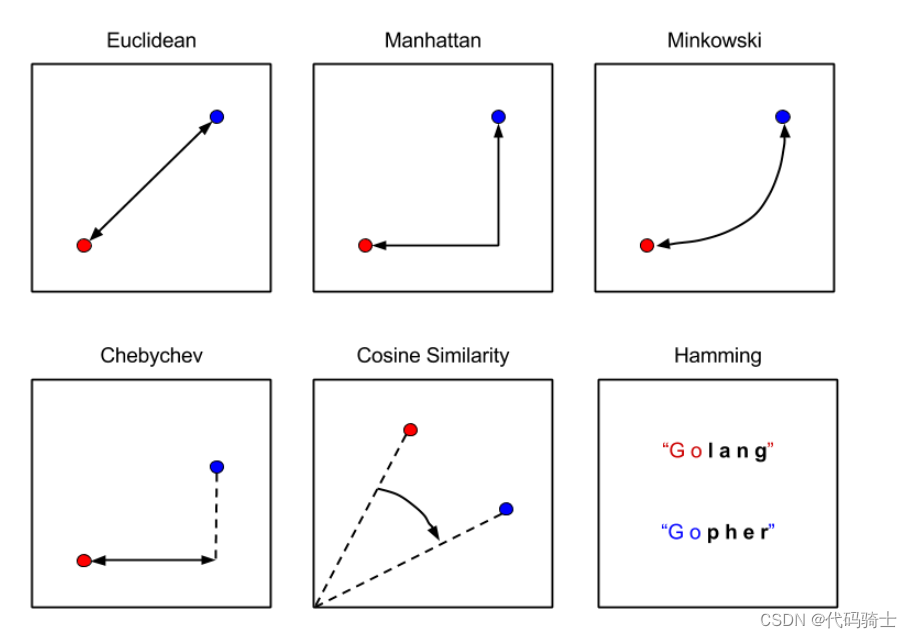
求距离差异的机器学习算法有很多,以下是一些常见的算法:
- - 欧氏距离(Euclidean Distance):欧氏距离是最容易直观理解的距离度量方法,我们小学、初中和高中接触到的两个点在空间中的距离一般都是指欧氏距离。
- - 曼哈顿距离(Manhattan Distance):曼哈顿距离是指在m维空间中两个点之间的绝对轴距总和,也就是两个点在各个坐标轴上差的绝对值之和。
- - 切比雪夫距离(Chebyshev Distance):切比雪夫距离是指两个点在m维空间中所在坐标轴上差的最大值。
- - 闵可夫斯基距离(Minkowski Distance):闵可夫斯基距离是一种通用的距离度量方法,它可以通过将欧几里得距离公式中的p参数取不同的值来定义不同类型的距离。
- - 余弦相似度(Cosine Similarity),是通过测量两个向量的夹角的余弦值来评估它们之间的相似性。其范围从-1(表示完全不相似)到+1(表示完全相同)。例如,在处理文本数据时,我们可以将每篇文档向量化,然后通过计算向量之间的余弦相似度来确定它们的相关性。在某些实现中,如sklearn库,提供了内置函数cosine_similarity()直接用来计算余弦相似性。
- - 海明距离(Hamming)则是一种测量两个等长字符串之间对应位置的不同字符的数量,通常用于比较二进制字符串。它的基本思想是,对于两个等长的字符串,对应位置上不同字符的个数就是它们的海明距离。海明距离同样也可以用于衡量其他类型的数据的相似性或差异性,比如将原始数据映射为二进制指纹后,就可以通过计算二进制指纹在相同位置上不同字符的个数来衡量数据的相似性或差异性。
距离算法应用:
欧氏距离、曼哈顿距离、切比雪夫距离、闵可夫斯基距离、余弦相似度和海明距离各自有其特定的应用场景和优缺点。
- 欧氏距离可能是最常见的一种距离度量方法,它定义为两个点之间的直线距离,通常用于表示实际空间中的距离。然而,欧氏距离并非尺度不变的,即所计算的距离可能会因元素的单位而产生偏斜。
- 曼哈顿距离,也称为城市街区距离,是另一种常用的距离度量方式,它是在一个网格状的城市中,从一个十字路口驾驶到另一个十字路口所需的最小距离。与欧氏距离不同,曼哈顿距离并不考虑各维度之间的方向,只计算其绝对值。
- 切比雪夫距离是由国际象棋中国王的走法启发而得的一种距离度量,它表示的是两个点之间的最小跳跃次数。
- 闵可夫斯基距离是对多个距离度量公式的概括性表述,它是一种灵活的距离定义方法,通过一个变参数p来改变距离计算方式。当p=1时,就是曼哈顿距离;当p=2时,就是欧氏距离;当p→∞时,就是切比雪夫距离。
- 余弦相似度是用两个向量夹角的余弦来衡量它们之间的相似性。如果将向量归一化为长度均为1的向量,则向量的内积也相同。两个方向完全相同的向量的余弦相似度为1,而两个彼此相对的向量的相似度为-1。
- 海明距离是一种衡量两个等长字符串之间对应位置的不同字符的数量的方式,通常用于比较二进制字符串。
详细公式:
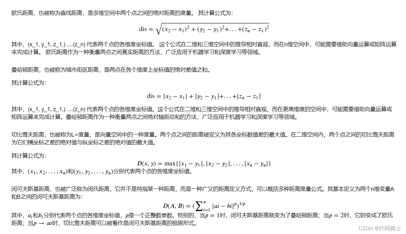

导入数据集
data=sns.load_dataset('iris')
划分特征变量和响应变量
X = data.drop(['species'], axis=1)
y = data['species']
创建模型评估得分
## Importing the model.
from sklearn.model_selection import StratifiedShuffleSplit, cross_val_score
from sklearn.neighbors import KNeighborsClassifier

## calling on the model oject.
knn = KNeighborsClassifier(metric='minkowski', p=2)#minkowski算法:p=1——曼哈顿,p=2——欧几里得
## knn classifier works by doing euclidian distance

## doing 10 fold staratified-shuffle-split cross validation
cv = StratifiedShuffleSplit(n_splits=10, test_size=.25, random_state=2)

accuracies = cross_val_score(knn, X,y, cv = cv, scoring='accuracy')
print ("Cross-Validation accuracy scores:{}".format(accuracies))
print ("Mean Cross-Validation accuracy score: {}".format(round(accuracies.mean(),3)))
Cross-Validation accuracy scores:[1. 0.97368421 0.94736842 0.97368421 0.97368421 1. 0.97368421 0.97368421 0.97368421 0.94736842] Mean Cross-Validation accuracy score: 0.974
调整模型参数K
## Search for an optimal value of k for KNN.
k_range = range(1,31)
k_scores = []
for k in k_range:
    knn = KNeighborsClassifier(n_neighbors=k)
    scores = cross_val_score(knn, X,y, cv = cv, scoring = 'accuracy')
    k_scores.append(scores.mean())
print("Accuracy scores are: {}\n".format(k_scores))
print ("Mean accuracy score: {}".format(np.mean(k_scores)))
Accuracy scores are: [0.9552631578947368, 0.9526315789473683, 0.9631578947368421, 0.9578947368421054, 0.9736842105263157, 0.9710526315789474, 0.9763157894736842, 0.968421052631579, 0.9763157894736842, 0.9605263157894737, 0.9736842105263159, 0.968421052631579, 0.976315789473684, 0.9631578947368421, 0.968421052631579, 0.9605263157894737, 0.9657894736842104, 0.9552631578947368, 0.9631578947368421, 0.9552631578947368, 0.9657894736842104, 0.9552631578947368, 0.9605263157894737, 0.9605263157894737, 0.9605263157894737, 0.9552631578947368, 0.9605263157894737, 0.9578947368421054, 0.9605263157894737, 0.9526315789473685] Mean accuracy score: 0.9631578947368421
绘制k与score的图像
from matplotlib import pyplot as plt
plt.plot(k_range, k_scores, 'bo',linestyle='dashed',linewidth=1,markersize=6)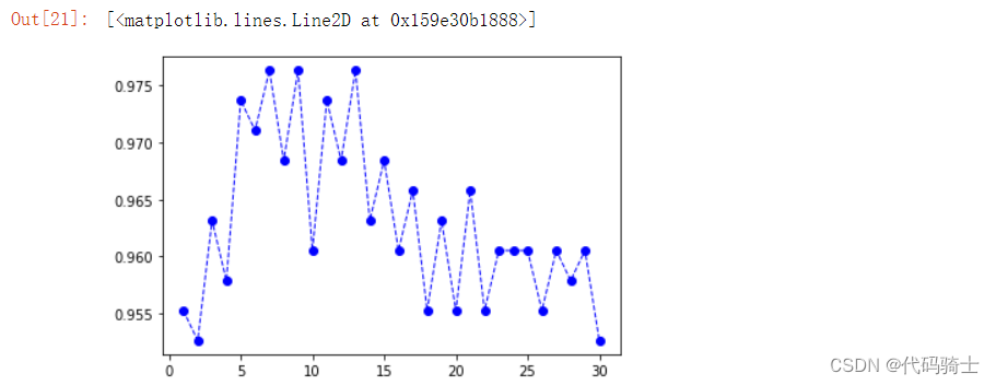
Grid search on KNN classifier
rid search on KNN classifier是指在K近邻(K-Nearest Neighbors,简称KNN)分类器上进行网格搜索(Grid Search)的过程。
KNN是一种基于实例的学习方法,它通过计算待分类样本与训练集中样本之间的距离,选取距离最近的K个邻居,然后根据这K个邻居的类别进行投票,得到待分类样本的类别。
网格搜索(Grid Search)是一种参数优化方法,用于在给定的参数范围内搜索最优的超参数组合。对于KNN分类器,常见的需要优化的超参数包括:K值(即选择多少个最近邻)、距离度量方法(如欧氏距离、曼哈顿距离等)、权重方法(如距离倒数、相等权重等)等。
在进行网格搜索时,会为每个超参数设定一个可能的值范围,然后遍历所有可能的超参数组合,对每个组合训练KNN分类器,并使用交叉验证(Cross Validation)等方法评估模型的性能。最后,选择性能最好的超参数组合作为模型的最终参数。
网格搜索(Grid Search)是一种调参技术,其基本思想是穷举遍历所有可能的超参数组合,从中找到使模型表现最优的那一组。这种算法的主要应用场景是机器学习中,用于选择模型的最优超参数。
在实际应用中,我们经常需要从一系列的超参数中选择一组最优的组合,用以提升模型的性能。如果超参数选择不恰当,可能会出现欠拟合或者过拟合的问题。这时候,就可以借助网格搜索的方法来进行处理。
具体操作流程为:首先,我们需要定义每一个超参数的可能取值范围;然后,网格搜索会在这些可能的取值范围内,按照预定的步长依次调整参数;接下来,针对每一种参数组合,实例化给定的模型,并使用交叉验证进行评估;最后,将平均得分最高的超参数组合作为最佳的选择,返回最优的模型对象。
from sklearn.model_selection import GridSearchCV
## trying out multiple values for k
k_range = range(1,31)
##
weights_options=['uniform','distance']
#
param = {'n_neighbors':k_range, 'weights':weights_options}
## Using startifiedShufflesplit.
cv = StratifiedShuffleSplit(n_splits=10, test_size=.30, random_state=15)
# estimator = knn, param_grid = param, n_jobs = -1 to instruct scikit learn to use all available processors.
grid = GridSearchCV(KNeighborsClassifier(), param,cv=cv,verbose = False, n_jobs=-1)
## Fitting the model.
grid.fit(X,y)
GridSearchCV(cv=StratifiedShuffleSplit(n_splits=10, random_state=15, test_size=0.3,
train_size=None),
error_score=nan,
estimator=KNeighborsClassifier(algorithm='auto', leaf_size=30,
metric='minkowski',
metric_params=None, n_jobs=None,
n_neighbors=5, p=2,
weights='uniform'),
iid='deprecated', n_jobs=-1,
param_grid={'n_neighbors': range(1, 31),
'weights': ['uniform', 'distance']},
pre_dispatch='2*n_jobs', refit=True, return_train_score=False,
scoring=None, verbose=False)
print(grid.best_score_)
print(grid.best_params_)
print(grid.best_estimator_)
0.9666666666666668
{'n_neighbors': 13, 'weights': 'distance'}
KNeighborsClassifier(algorithm='auto', leaf_size=30, metric='minkowski',
metric_params=None, n_jobs=None, n_neighbors=13, p=2,
weights='distance')
### Using the best parameters from the grid-search.
knn_grid= grid.best_estimator_
knn_grid.score(X,y)
1.0
处理过拟合可以采取以下策略:
- 1. 增加数据量:这是解决过拟合最常用的方法。如果有更多的训练数据,模型将有更多的信息进行学习和理解,从而降低过拟合的风险。
- 2. 减少特征数量:有时,输入的特征过多会导致模型过于复杂,从而引发过拟合。可以考虑通过特征选择或特征提取的方式减少特征的数量。
- 3. 正则化:正则化是一种通过对模型参数添加惩罚项的方式来限制参数的大小,防止模型变得过于复杂而导致过拟合。
- 4. 采用深度学习方法:深度学习可以通过增加网络的深度和宽度等手段来提高模型的表达能力,从而减轻过拟合的问题。
- 5. 采用集成学习方法:集成学习可以通过组合多个基学习器来提高模型的性能和泛化能力,从而减轻过拟合的问题。
- 6. 后剪枝:这是一种在构建完整的决策树后,通过反向修剪来删除那些对泛化性能影响较小的子树和叶节点的方法,以达到减少模型复杂度、避免过拟合的目的。
Using RandomizedSearchCV
RandomizedSearchCV是scikit-learn库中的一个类,用于执行随机搜索交叉验证。它的主要目的是在超参数空间中寻找最优的超参数组合,以提高模型的性能。
随机搜索与网格搜索不同,网格搜索会尝试所有可能的超参数组合,而随机搜索则从给定的超参数分布中随机选择一定数量的组合进行评估。这种方法可以大大减少计算时间,特别是当超参数空间很大时。
使用RandomizedSearchCV的基本步骤如下:
- 导入所需的库和模块。
- 定义一个包含超参数的字典,例如
param_distributions。 - 创建一个
RandomizedSearchCV对象,传入模型、超参数字典、评分指标等参数。 - 使用
fit方法对数据进行拟合。 - 使用
predict方法进行预测。 - 使用
best_params_属性获取最佳超参数组合。 - 使用
best_score_属性获取最佳模型的评分。
from sklearn.model_selection import RandomizedSearchCV
## trying out multiple values for k
k_range = range(1,31)
##
weights_options=['uniform','distance']
#
param = {'n_neighbors':k_range, 'weights':weights_options}
## Using startifiedShufflesplit.
cv = StratifiedShuffleSplit(n_splits=10, test_size=.30)
# estimator = knn, param_grid = param, n_jobs = -1 to instruct scikit learn to use all available processors.
## for RandomizedSearchCV,
grid = RandomizedSearchCV(KNeighborsClassifier(), param,cv=cv,verbose = False, n_jobs=-1, n_iter=40)
## Fitting the model.
grid.fit(X,y)
RandomizedSearchCV(cv=StratifiedShuffleSplit(n_splits=10, random_state=None, test_size=0.3,
train_size=None),
error_score=nan,
estimator=KNeighborsClassifier(algorithm='auto',
leaf_size=30,
metric='minkowski',
metric_params=None,
n_jobs=None, n_neighbors=5,
p=2, weights='uniform'),
iid='deprecated', n_iter=40, n_jobs=-1,
param_distributions={'n_neighbors': range(1, 31),
'weights': ['uniform', 'distance']},
pre_dispatch='2*n_jobs', random_state=None, refit=True,
return_train_score=False, scoring=None, verbose=False)
print (grid.best_score_)
print (grid.best_params_)
print(grid.best_estimator_)0.9844444444444445
{'weights': 'distance', 'n_neighbors': 13}
KNeighborsClassifier(algorithm='auto', leaf_size=30, metric='minkowski',
metric_params=None, n_jobs=None, n_neighbors=13, p=2,
weights='distance')
### Using the best parameters from the grid-search.
knn_ran_grid = grid.best_estimator_
knn_ran_grid.score(X,y)1.0
处理过拟合可以采取以下策略:
- 1. 增加数据量:这是解决过拟合最常用的方法。如果有更多的训练数据,模型将有更多的信息进行学习和理解,从而降低过拟合的风险。
- 2. 减少特征数量:有时,输入的特征过多会导致模型过于复杂,从而引发过拟合。可以考虑通过特征选择或特征提取的方式减少特征的数量。
- 3. 正则化:正则化是一种通过对模型参数添加惩罚项的方式来限制参数的大小,防止模型变得过于复杂而导致过拟合。
- 4. 采用深度学习方法:深度学习可以通过增加网络的深度和宽度等手段来提高模型的表达能力,从而减轻过拟合的问题。
- 5. 采用集成学习方法:集成学习可以通过组合多个基学习器来提高模型的性能和泛化能力,从而减轻过拟合的问题。
- 6. 后剪枝:这是一种在构建完整的决策树后,通过反向修剪来删除那些对泛化性能影响较小的子树和叶节点的方法,以达到减少模型复杂度、避免过拟合的目的。
P24-Support Vector Machine建模
https://www.youtube.com/watch?v=Jlm-80v70HY&list=PLGkfh2EpdoKU3OssXkTl3y7c9tw7jjvHm&index=31
支持向量机(Support Vector Machine, SVM)是一种监督式机器学习算法,可用于分类或回归问题。然而,它主要用于分类问题。在该算法中,我们将每个数据项绘制为n维空间中的点(其中n是特征的数量),每个特征的值为特定坐标的值。然后,我们通过找到区分两个类别非常好的超平面来进行分类。一般来说,当特征数量非常大时,SVM表现非常好。例如,在词袋模型中进行文本分类。
就SVM而言,在以下情况下它是一种合适的分类器:
1) 当特征数量(变量)和训练数据的数量非常大(例如数百万个特征和数百万个实例(数据))。
2) 当问题的稀疏性非常高时,即大多数特征的值为0。
3) 它最适合文档分类问题,其中稀疏性高且特征/实例也很多。
4) 它还可以很好地解决图像分类、基因分类、药物歧义等问题,其中特征数量很高。它是最佳选择之一,原因如下:
1、 它使用核技巧。
2、它是机器学习中基于最优边界的分类技术。
3、有许多算法被提出,利用问题结构和其他较小的因素,如优化期间的问题缩小等。
from IPython.display import Image
Image(filename='C:\\Users\\86185\\Desktop\\TempDesktop\\研究内容\\Python学习\\Py机深文字教程+源码\\LessonPythonCode-main\\Lesson24-SVM.png')
#C:\\Users\\86185\\Desktop\\TempDesktop\\研究内容\\Python学习\\Py机深文字教程+源码\\LessonPythonCode-main
from IPython.display import Image
Image(filename='C:\\Users\\86185\\Desktop\\TempDesktop\\研究内容\\Python学习\\Py机深文字教程+源码\\LessonPythonCode-main\\Lesson24-SVM1.png')
#Image(filename='D:\\python\\Project0-Python-MachineLearning\\Lesson24-SVM1.png')

(1)SVM 对于 Iris 数据集的处理
导入函数库
import numpy as np # linear algebra
import pandas as pd # data processing, CSV file I/O (e.g. pd.read_csv)
import matplotlib.pyplot as plt
import seaborn as sns
from sklearn.preprocessing import PolynomialFeatures, StandardScaler
from sklearn.svm import LinearSVC
from sklearn.svm import SVC
from sklearn.model_selection import train_test_split加载数据集
from sklearn import datasets #参考第11课,19课,20课
iris = datasets.load_iris()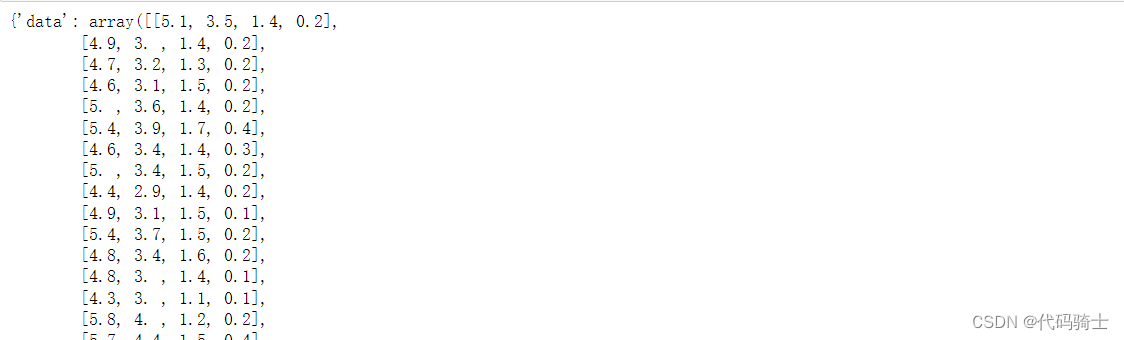
重新定义数据集
X = iris['data'][:,(2,3)]
scaler = StandardScaler()
Xstan = scaler.fit_transform(X)
data = pd.DataFrame(data=Xstan, columns=['petal length','petal width'])
data['target'] = iris['target']
data = data[data['target']!=2] # we will only focus on Iris-setosa and Iris-Versicolor
data
sns.lmplot函数是Seaborn库中的一个绘图函数,它结合了基础绘图与基于数据建立回归模型的特性。这个函数的主要目标是创建一个方便用户拟合数据集回归模型的绘图方法。
在lmplot中,你可以使用'hue'、'col'、'row'参数来控制绘图变量。例如,如果你想要根据某个特性对数据点进行着色,可以使用'hue'参数;如果你想要根据另一个特性将数据分组并在不同的列中绘制,可以使用'col'参数;同样,如果你想要根据第三个特性将数据在不同的行中绘制,可以使用'row'参数。
此外,lmplot还允许你通过调整模型参数来改变拟合的模型类型,这些模型包括:顺序(order)、逻辑斯蒂(logistic)、lowess、鲁棒(robust)和对数(logx)等。
sns.lmplot(x='petal length',y='petal width',hue='target',data=data, fit_reg=False, legend=False)
plt.legend(['Iris-Setosa','Iris-Versicolor'], fontsize = 14)
plt.xlabel('petal length (scaled)', fontsize = 18)
plt.ylabel('petal width (scaled)', fontsize = 18)
plt.show()
svc = LinearSVC(C=1,loss="hinge")#C参数控制正则化强度,loss参数指定损失函数类型为hinge(即“感知器”损失)。
svc.fit(data[['petal length','petal width']].values,data['target'].values)获取模型参数,求出decision boundary和margin
# get the parameters
w0,w1 = svc.coef_[0]#模型洗漱个数由特征个数而定(类比多元线性回归)—— y = w0x0+w1x1+b
b = svc.intercept_[0]
x0 = np.linspace(-1.7, 0.7, num=100)
# decision boundary
x1_decision = -b/w1 - w0/w1*x0# 0 = w0x0+w1x1+b
# +1 margin
x1_plus = x1_decision + 1/w1# 1 = w0x0+w1x1+b
# -1 margin
x1_minus = x1_decision - 1/w1# -1 = w0x0+w1x1+b 绘制图像
sns.lmplot(x='petal length',y='petal width',hue='target',data=data, fit_reg=False, legend=False)
plt.plot(x0,x1_decision, color='grey')
plt.plot(x0,x1_plus,x0,x1_minus,color='grey', linestyle='--')
plt.legend(['decision boundary','margin','margin','Iris-Setosa','Iris-Versicolor'], fontsize = 14, loc='center left', bbox_to_anchor=(1.05,0.5))
plt.xlabel('petal length (scaled)', fontsize = 18)
plt.ylabel('petal width (scaled)', fontsize = 18)
plt.title('C = 1', fontsize = 20)
plt.ylim(-1.6,1)
plt.xlim(-1.7,0.8)
plt.show()
调整参数C控制正则化强度
svc = LinearSVC(C=1000,loss="hinge") # let's change C to a much larger value
svc.fit(data[['petal length','petal width']].values,data['target'].values)
# get the parameters
w0,w1 = svc.coef_[0]
b = svc.intercept_[0]
x0 = np.linspace(-1.7, 0.7, num=100)
# decision boundary
x1_decision = -b/w1 - w0/w1*x0
# +1 margin
x1_plus = x1_decision + 1/w1
# -1 margin
x1_minus = x1_decision - 1/w1绘图
sns.lmplot(x='petal length',y='petal width',hue='target',data=data, fit_reg=False, legend=False)
plt.plot(x0,x1_decision, color='grey')
plt.plot(x0,x1_plus,x0,x1_minus,color='grey', linestyle='--')
plt.legend(['decision boundary','margin','margin','Iris-Setosa','Iris-Versicolor'], fontsize = 14, loc='center left', bbox_to_anchor=(1.05,0.5))
plt.xlabel('petal length (scaled)', fontsize = 18)
plt.ylabel('petal width (scaled)', fontsize = 18)
plt.title('C = 1000', fontsize = 20)
plt.ylim(-1.6,1)
plt.xlim(-1.7,0.8)
plt.show()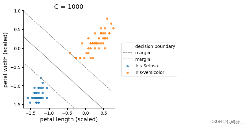
(2)SVM 对于 弯月数据集的处理
from sklearn.datasets import make_moons
X,y=make_moons(noise=0.1, random_state=2) # fix random_state to make sure it produces the same dataset everytime. Remove it if you want randomized dataset.
data = pd.DataFrame(data = X, columns=['x1','x2'])
data['y']=y
data.head()
sns.lmplot(x='x1',y='x2',hue='y',data=data, fit_reg=False, legend=True, height=4, aspect=4/3)
plt.xlabel('x1', fontsize = 18)
plt.ylabel('x2', fontsize = 18)
plt.show()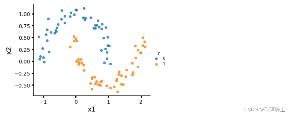
# tranform the features, here we use a 3rd degree polynomials
print('Shape of X before tranformation:', X.shape)
poly = PolynomialFeatures(degree = 3, include_bias=False)
Xpoly = poly.fit_transform(X)
print('Shape of X aftere tranformation:', Xpoly.shape)Shape of X before tranformation: (100, 2) Shape of X aftere tranformation: (100, 9)
数据标准化
# standardize the data
scaler = StandardScaler()
Xpolystan = scaler.fit_transform(Xpoly)svm_clf = LinearSVC(C=10,loss='hinge',max_iter=10000)
svm_clf.fit(Xpolystan,y)
print(svm_clf.intercept_, svm_clf.coef_)[0.14733956] [[-1.48196089 -0.38932002 -3.63173089 -0.24404565 0.84163819 6.20766925 -0.9820019 0.70831626 -1.94868814]]
# preparing to plot decision boundary of the classifier
def make_meshgrid(x, y, h=.02):
x_min, x_max = x.min() - 1, x.max() + 1
y_min, y_max = y.min() - 1, y.max() + 1
xx, yy = np.meshgrid(np.arange(x_min, x_max, h), np.arange(y_min, y_max, h))
return xx, yy# create grids
X0, X1 = X[:, 0], X[:, 1]
xx0, xx1 = make_meshgrid(X0, X1)
# polynomial transformation and standardization on the grids
xgrid = np.c_[xx0.ravel(), xx1.ravel()]
xgridpoly = poly.transform(xgrid)
xgridpolystan = scaler.transform(xgridpoly)
# prediction
Z = xgridpolystan.dot(svm_clf.coef_[0].reshape(-1,1)) + svm_clf.intercept_[0] # wx + b
#Z = svm_clf.predict(xgridpolystan)
Z = Z.reshape(xx0.shape)# plotting prediction contours - decision boundary (Z=0), and two margins (Z = 1 or -1)
sns.lmplot(x='x1',y='x2',hue='y',data=data, fit_reg=False, legend=True, height=4, aspect=4/3)
CS=plt.contour(xx0, xx1, Z, alpha=0.5, levels=[-1,0,1])
plt.clabel(CS, inline=1,levels=[-1.0,0,1.0], fmt='%1.1f', fontsize=12, manual=[(1.5,0.3),(0.5,0.0),(-0.5,-0.2)])
#
plt.xlim(-1.2,2.2)
plt.ylim(-1,1.5)
plt.title('C=10', fontsize = 20)
plt.xlabel('x1', fontsize = 18)
plt.ylabel('x2', fontsize = 18)
plt.show()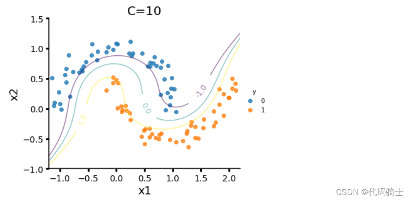
svm_clf = LinearSVC(C=1000,loss='hinge',max_iter=10000)
svm_clf.fit(Xpolystan,y)
# prediction
Z = xgridpolystan.dot(svm_clf.coef_[0].reshape(-1,1)) + svm_clf.intercept_[0] # wx + b
#Z = svm_clf.predict(xgridpolystan)
Z = Z.reshape(xx0.shape)
# plotting prediction contours - decision boundary (Z=0), and two margins (Z = 1 or -1)
sns.lmplot(x='x1',y='x2',hue='y',data=data, fit_reg=False, legend=True, height=4, aspect=4/3)
CS=plt.contour(xx0, xx1, Z, alpha=0.5, levels=[-1,0,1])
plt.clabel(CS, inline=1,levels=[-1.0,0,1.0], fmt='%1.1f', fontsize=12, manual=[(1.5,0.1),(0.5,0.0),(-0.5,0.0)])
plt.xlim(-1.2,2.2)
plt.ylim(-1,1.5)
plt.title('C=1000', fontsize = 20)
plt.xlabel('x1', fontsize = 18)
plt.ylabel('x2', fontsize = 18)
plt.show()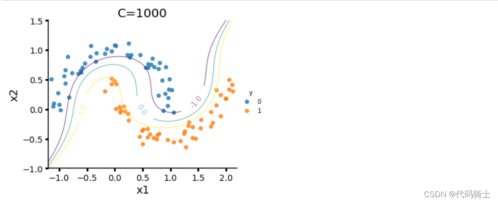
from sklearn.svm import SVCscaler = StandardScaler()
Xstan = scaler.fit_transform(X)
svm_clf = SVC(kernel='poly', degree=3, C=10, coef0=1)
svm_clf.fit(Xstan,y)
# create grids
X0, X1 = X[:, 0], X[:, 1]
xx0, xx1 = make_meshgrid(X0, X1)
# standardization on the grids
xgrid = np.c_[xx0.ravel(), xx1.ravel()]
xgridstan = scaler.transform(xgrid)
# prediction
Z = svm_clf.predict(xgridstan)
Z = Z.reshape(xx0.shape)
# plotting prediction contours - decision boundary (Z=0), and two margins (Z = 1 or -1)
sns.lmplot(x='x1',y='x2',hue='y',data=data, fit_reg=False, legend=True, height=4, aspect=4/3)
plt.contourf(xx0, xx1, Z, alpha=0.5)
plt.xlim(-1.2,2.2)
plt.ylim(-1,1.5)
plt.title('C=10', fontsize = 20)
plt.xlabel('x1', fontsize = 18)
plt.ylabel('x2', fontsize = 18)
plt.show()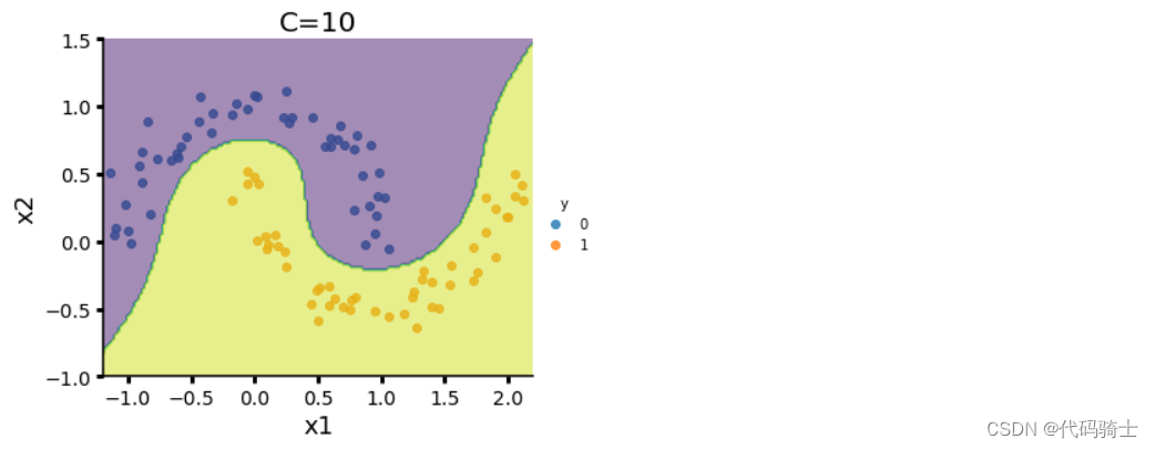
(3)SVM 对于 direct marketing campaigns (phone calls)数据集的处理
data = pd.read_csv('Lesson24-bank-additional-full.csv',sep=';') # note that the delimiter for this dataset is ";"
data = data.drop('duration',axis=1) # as recommended by the dataset description, we will drop the last contact duration values.header = ['age','campaign','pdays','previous','emp.var.rate','cons.price.idx','cons.conf.idx','euribor3m','nr.employed']
data.hist(column=header,figsize=(10,10))
plt.subplots_adjust(wspace = 0.5, hspace = 0.5)
plt.show()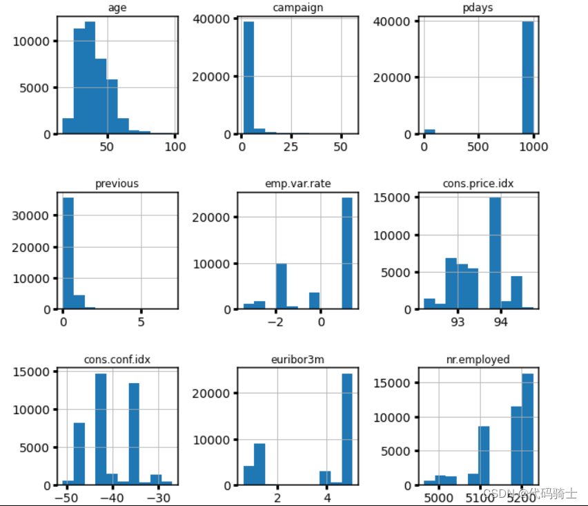
实现数据类型转换——map()函数
data['poutcome'] = data['poutcome'].map({'failure': -1,'nonexistent': 0,'success': 1})data['default'] = data['default'].map({'yes': -1,'unknown': 0,'no': 1})
data['housing'] = data['housing'].map({'yes': -1,'unknown': 0,'no': 1})
data['loan'] = data['loan'].map({'yes': -1,'unknown': 0,'no': 1})实现数据类型转换——get_dummies()函数
nominal = ['job','marital','education','contact','month','day_of_week']
dataProcessed = pd.get_dummies(data,columns=nominal)dataProcessed['y']=dataProcessed['y'].map({'yes': 1,'no': 0})
dataProcessed.head()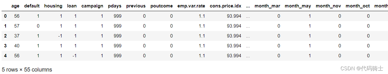
from sklearn.model_selection import train_test_split# raw data
X = dataProcessed.drop('y', axis=1).values
y = dataProcessed['y'].values
# split, random_state is used for repeatable results, you should remove it if you are running your own code.
X_train, X_test, y_train, y_test = train_test_split(X, y, test_size=0.30, random_state=42)
print('X train size: ', X_train.shape)
print('y train size: ', y_train.shape)
print('X test size: ', X_test.shape)
print('y test size: ', y_test.shape)X train size: (28831, 54) y train size: (28831,) X test size: (12357, 54) y test size: (12357,)
# column index of numeric variables
idx_numeric=[0,4,5,6,8,9,10,11,12]
##print(dataProcessed.columns[idx])
# standardize numeric variables only
scaler = StandardScaler()
X_train[:,idx_numeric]=scaler.fit_transform(X_train[:,idx_numeric])
X_test[:,idx_numeric]=scaler.transform(X_test[:,idx_numeric])from sklearn.model_selection import GridSearchCVtuned_parameters = [{'kernel': ['rbf'], 'gamma': [0.1],
'C': [1]},
{'kernel': ['linear'], 'C': [1]}]
clf = GridSearchCV(SVC(), tuned_parameters, cv=5, scoring='precision')
clf.fit(X_train, y_train)print(clf.cv_results_){'mean_fit_time': array([107.24569249, 564.51672297]), 'std_fit_time': array([ 31.20087915, 183.30460925]), 'mean_score_time': array([5.88282857, 6.32607164]), 'std_score_time': array([1.72741235, 1.73930083]), 'param_C': masked_array(data=[1, 1],
mask=[False, False],
fill_value='?',
dtype=object), 'param_gamma': masked_array(data=[0.1, --],
mask=[False, True],
fill_value='?',
dtype=object), 'param_kernel': masked_array(data=['rbf', 'linear'],
mask=[False, False],
fill_value='?',
dtype=object), 'params': [{'C': 1, 'gamma': 0.1, 'kernel': 'rbf'}, {'C': 1, 'kernel': 'linear'}], 'split0_test_score': array([0.66044776, 0.64186047]), 'split1_test_score': array([0.64081633, 0.61320755]), 'split2_test_score': array([0.66396761, 0.64878049]), 'split3_test_score': array([0.68325792, 0.65128205]), 'split4_test_score': array([0.69731801, 0.67924528]), 'mean_test_score': array([0.66916153, 0.64687517]), 'std_test_score': array([0.01948257, 0.02111649]), 'rank_test_score': array([1, 2])}
print('The best model is: ', clf.best_params_)
print('This model produces a mean cross-validated score (precision) of', clf.best_score_)The best model is: {'C': 1, 'gamma': 0.1, 'kernel': 'rbf'}
This model produces a mean cross-validated score (precision) of 0.6691615250551093
from sklearn.metrics import precision_score, accuracy_scorey_true, y_pred = y_test, clf.predict(X_test)
print('precision on the evaluation set: ', precision_score(y_true, y_pred))
print('accuracy on the evaluation set: ', accuracy_score(y_true, y_pred))precision on the evaluation set: 0.647834274952919 accuracy on the evaluation set: 0.9002994254268836
P25-Bayes贝叶斯识别Spam Email垃圾邮件
https://www.youtube.com/watch?v=8CBRiymMrzs&list=PLGkfh2EpdoKU3OssXkTl3y7c9tw7jjvHm&index=25
贝叶斯定理与公式

举例理解贝叶斯公式
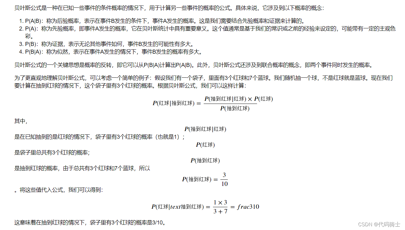
贝叶斯的分类

(1)伯努利朴素贝叶斯
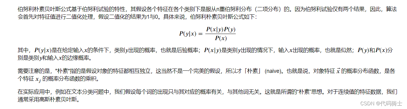
(2)多项式朴素贝叶斯
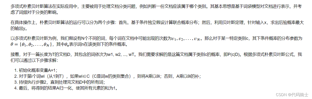
(3)高斯朴素贝叶斯
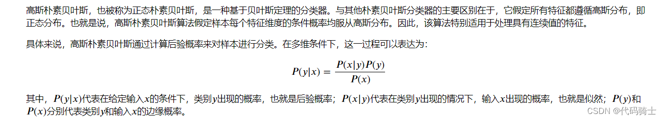
from IPython.display import Image
Image(filename='C:\\Users\\86185\\Desktop\\TempDesktop\\研究内容\\Python学习\\Py机深文字教程+源码\\LessonPythonCode-main\\Lesson25-card1.png')
#C:\\Users\\86185\\Desktop\\TempDesktop\\研究内容\\Python学习\\Py机深文字教程+源码\\LessonPythonCode-main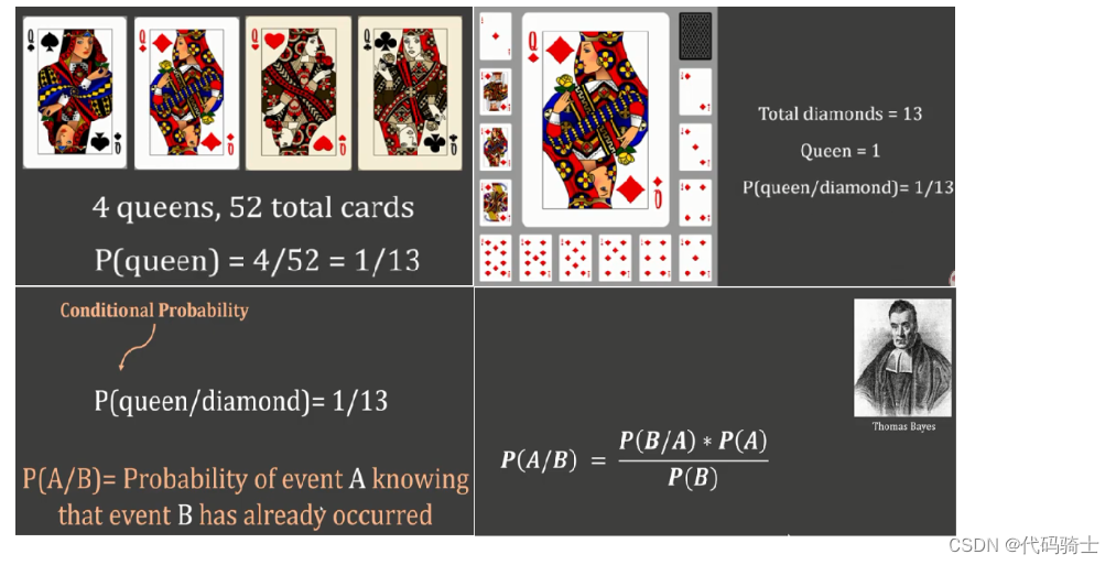
from IPython.display import Image
#Image(filename='D:\\python\\Project0-Python-MachineLearning\\Lesson25-card2.png')
Image(filename='C:\\Users\\86185\\Desktop\\TempDesktop\\研究内容\\Python学习\\Py机深文字教程+源码\\LessonPythonCode-main\\Lesson25-card2.png')
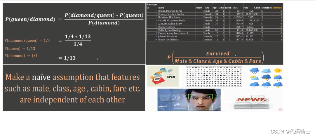
(1)应用Gaussian Naive Bayes预测沉船存活人数
import pandas as pd
#df = pd.read_csv("Lesson18-titanic.csv")
df = pd.read_csv("C:\\Users\\86185\\Desktop\\TempDesktop\\研究内容\\Python学习\\Py机深文字教程+源码\\seaborn-data-master\\raw\\titanic.csv")
#C:\\Users\\86185\\Desktop\\TempDesktop\\研究内容\\Python学习\\Py机深文字教程+源码\\seaborn-data-master\\raw\\titanic.csv
#C:\Users\86185\Desktop\TempDesktop\研究内容\Python学习\Py机深文字教程+源码\LessonPythonCode-main\Lesson21-titanic_test.csv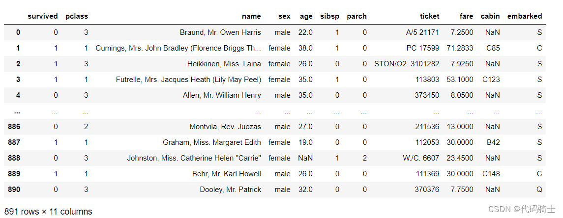
df.drop(['name','sibsp','parch','ticket','cabin','embarked'],axis='columns',inplace=True)
X = df.drop('survived',axis='columns')
y = df["survived"]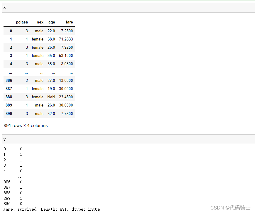
dummies = pd.get_dummies(X.sex)
X = pd.concat([X,dummies],axis='columns')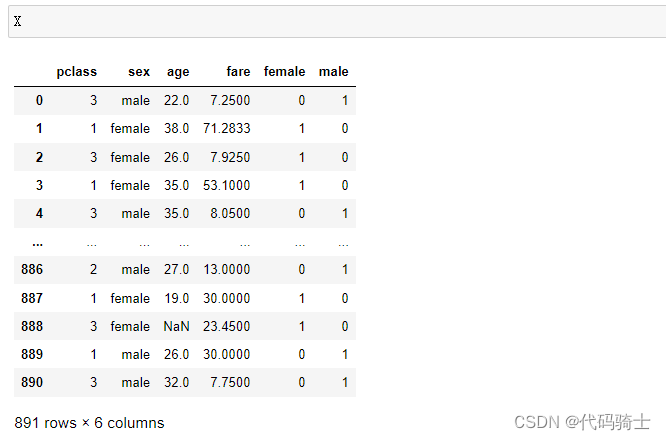
X.drop(['sex','female'],axis='columns',inplace=True)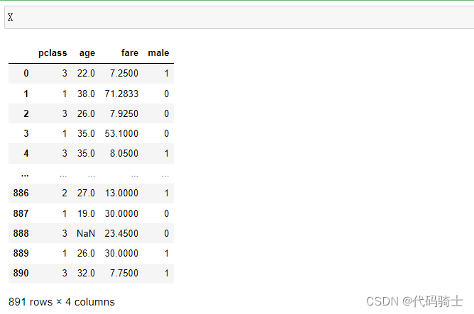
X.columns[X.isna().any()]Index(['age'], dtype='object')
X['age'].isnull().sum() #对于Age更深入的处理请参考第18课和21课177
X.age = X.age.fillna(X.age.mean())#用平均值填补空值from sklearn.model_selection import train_test_split
X_train, X_test, y_train, y_test = train_test_split(X,y,test_size=0.3)from sklearn.naive_bayes import GaussianNB
model = GaussianNB()model.fit(X_train,y_train)GaussianNB()
model.score(X_test,y_test)0.7873134328358209
X_test[0:10]
y_test[0:10]
model.predict(X_test[0:10])array([1, 1, 1, 0, 0, 0, 0, 0, 0, 0], dtype=int64)
model.predict_proba(X_test[:10])array([[0.45929949, 0.54070051],
[0.19830182, 0.80169818],
[0.43448283, 0.56551717],
[0.95974509, 0.04025491],
[0.95889759, 0.04110241],
[0.96417793, 0.03582207],
[0.96317246, 0.03682754],
[0.95804759, 0.04195241],
[0.64789556, 0.35210444],
[0.90121722, 0.09878278]])
from sklearn.model_selection import cross_val_score
cross_val_score(GaussianNB(),X_train, y_train, cv=5)array([0.736 , 0.776 , 0.768 , 0.75806452, 0.81451613])
from sklearn.metrics import classification_report
print(classification_report(y_test[0:10],model.predict(X_test[0:10]))) precision recall f1-score support
0 1.00 0.88 0.93 8
1 0.67 1.00 0.80 2
accuracy 0.90 10
macro avg 0.83 0.94 0.87 10
weighted avg 0.93 0.90 0.91 10
(2)应用Multinomial Naive Bayes处理垃圾邮件
df1 = pd.read_csv("Lesson25-spam_ham_dataset.csv")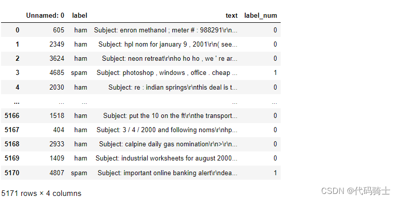
df1 = df1.drop(df1.columns[[0, 1]], axis=1) 
df1.groupby('label_num').describe()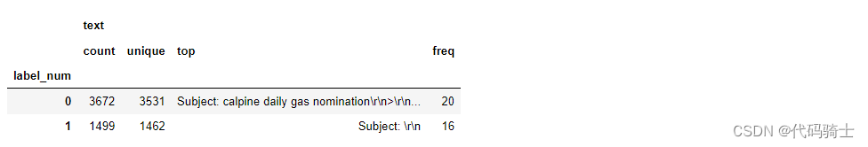
from sklearn.model_selection import train_test_split
X_train, X_test, y_train, y_test = train_test_split(df1.text,df1.label_num)from sklearn.feature_extraction.text import CountVectorizer
v = CountVectorizer()
X_train_T = v.fit_transform(X_train.values)#把字符串转换成向量
X_train_T.toarray()[:3]array([[0, 5, 0, ..., 0, 0, 0],
[0, 0, 0, ..., 0, 0, 0],
[0, 0, 0, ..., 0, 0, 0]], dtype=int64)
插曲:CountVectorizer 举例说明
from sklearn.feature_extraction.text import CountVectorizercorpus = [
'This is the first document.',
'This document is the second document.',
'And this is the third one.',
'Is this the first document?',
]vectorizer = CountVectorizer()X = vectorizer.fit_transform(corpus)print(vectorizer.get_feature_names())['and', 'document', 'first', 'is', 'one', 'second', 'the', 'third', 'this']
print(X.toarray())[[0 1 1 1 0 0 1 0 1] [0 2 0 1 0 1 1 0 1] [1 0 0 1 1 0 1 1 1] [0 1 1 1 0 0 1 0 1]]
原理剖析:
将corpus数组中的词提取出来(不重复),
根据每句话中词出现的个数,给对应位置的数组赋值,出现一次赋值1,出现两次赋值2,没出现过赋值0。
因此,对于上面的提取的基础词(字符表):
['and', 'document', 'first', 'is', 'one', 'second', 'the', 'third', 'this']
这句话
This is the first document.
代表的数组(向量)是:
[0,1,1,1,0,0,1,0,1]
二维向量
vectorizer2 = CountVectorizer(analyzer='word', ngram_range=(2, 2))X2 = vectorizer2.fit_transform(corpus)print(vectorizer2.get_feature_names())['and this', 'document is', 'first document', 'is the', 'is this', 'second document', 'the first', 'the second', 'the third', 'third one', 'this document', 'this is', 'this the']
print(X2.toarray())[[0 0 1 1 0 0 1 0 0 0 0 1 0] [0 1 0 1 0 1 0 1 0 0 1 0 0] [1 0 0 1 0 0 0 0 1 1 0 1 0] [0 0 1 0 1 0 1 0 0 0 0 0 1]]
插曲:CountVectorizer 举例说明结束
from sklearn.naive_bayes import MultinomialNB
model = MultinomialNB()
model.fit(X_train_T,y_train)MultinomialNB()
emails = [
'Hey mohan, can we get together to watch footbal game tomorrow?',
'Upto 20% discount on parking, exclusive offer just for you. Dont miss this reward!'
]
emails_T = v.transform(emails)
model.predict(emails_T)array([0, 1], dtype=int64)
X_test_T = v.transform(X_test)
model.score(X_test_T, y_test)0.9737045630317092
Sklearn Pipeline 老外真的很懒,发明了pipeline替代transform几行代码
from sklearn.pipeline import Pipeline
clf = Pipeline([
('vectorizer', CountVectorizer()),
('nb', MultinomialNB())
])clf.fit(X_train, y_train)Pipeline(steps=[('vectorizer', CountVectorizer()), ('nb', MultinomialNB())])
clf.score(X_test,y_test)0.9737045630317092
clf.predict(emails)array([0, 1], dtype=int64)
P26-Votingclassifier及11种算法全自动建模预测输出结果之完整源代码
https://www.youtube.com/watch?v=5j8SfEoTRYI&list=PLGkfh2EpdoKU3OssXkTl3y7c9tw7jjvHm&index=30
代码参考P21
P27-无监督学习K Means Clustering
https://www.youtube.com/watch?v=embAwRoe_-w&list=PLGkfh2EpdoKU3OssXkTl3y7c9tw7jjvHm&index=24
K-Means Clustering是什么?
K-Means Clustering,即K均值聚类算法,是一种迭代求解的聚类分析算法。其基本思想是“物以类聚,人以群分”,也就是将数据分为K组,其中K是我们预先指定的分组数量。算法执行过程如下:首先,从数据集中随机选取K个对象作为初始的聚类中心;然后,计算每个对象与各个种子聚类中心之间的距离;最后,根据每个对象与各聚类中心的距离,将每个对象分配给距离它最近的聚类中心。
此算法的主要目标是最小化同一个簇内的差异和最大化不同簇之间的差异,这可以用误差平方和来描述,它是K-Means算法的目标函数。
需要注意的是,虽然K-Means算法广泛应用于各种领域,但它也有自身的局限性。例如,它需要事先知道簇的数量K,对初始聚类中心的选择敏感,可能陷入局部最优解,以及对于非球形簇和大小不一的簇的适应性较差。
K值应该怎样选取?
K-Means聚类算法中,确定最佳的K值是一个重要的步骤。常见的一种方法是肘部法则(Elbow Method)。具体来说,先假设K=1,即所有数据点都聚合为一类,然后找到这个类别的中心点。接着逐步增加K值,让计算机进行计算,每次计算都会得到一个WSS(within cluster sum of squares),即各个点到簇中心的距离的平方和。通过绘制K值与WSS之间的关系图,也就是肘部图,可以观察到当K值增加时,WSS的变化情况。在K值较小的时候,WSS会快速下降;当K值继续增大时,WSS的下降速度会明显减慢,这个过程在图形上形成了一个肘部形状。通常认为,当K值达到使得WSS下降幅度开始平缓的那个点时,即肘部的位置,就是最佳的K值。
此外,还有其他一些方法可以用来确定K值,例如间隔统计量(Gap Statistic)、轮廓系数(Silhouette Coefficient)和Canopy算法等。这些方法各有优劣,可以根据实际的数据和需求来选择适合的方法。
算法介绍:
from IPython.display import Image
Image(filename='C:\\Users\\86185\\Desktop\\TempDesktop\\研究内容\\Python学习\\Py机深文字教程+源码\\LessonPythonCode-main\\Lesson27-cluster.png')
#C:\\Users\\86185\\Desktop\\TempDesktop\\研究内容\\Python学习\\Py机深文字教程+源码\\LessonPythonCode-main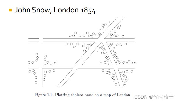
from IPython.display import Image
Image(filename='C:\\Users\\86185\\Desktop\\TempDesktop\\研究内容\\Python学习\\Py机深文字教程+源码\\LessonPythonCode-main\\Lesson27-Snow-cholera-map.jpg')
from IPython.display import Image
Image(filename='C:\\Users\\86185\\Desktop\\TempDesktop\\研究内容\\Python学习\\Py机深文字教程+源码\\LessonPythonCode-main\\Lesson27-Snow-cholera-map1.jpg')
from IPython.display import Image
Image(filename='C:\\Users\\86185\\Desktop\\TempDesktop\\研究内容\\Python学习\\Py机深文字教程+源码\\LessonPythonCode-main\\Lesson27-Elbow method.png')
from IPython.display import Image
Image(filename='C:\\Users\\86185\\Desktop\\TempDesktop\\研究内容\\Python学习\\Py机深文字教程+源码\\LessonPythonCode-main\\Lesson27-k-means-steps.png')
from sklearn.cluster import KMeans
import pandas as pd
from sklearn.preprocessing import MinMaxScaler
from matplotlib import pyplot as plt
%matplotlib inlineMinMaxScaler(feature_range = (0, 1)) 会将列中的每个值按比例转换为 [0,1] 范围内的值。将其作为第一个缩放器选项来转换特征,因为它会保留数据集的形状(无失真)。
StandardScaler() 会将列中的每个值转换为均值为0、标准差为1的范围,即通过减去均值并除以标准差对每个值进行归一化。如果您知道数据分布是正态的,请使用 StandardScaler。
当使用 MinMaxScaler 时,它也被称为归一化,它会将所有值转换为范围在 (0 到 1) 之间的值,公式为 x = [(value - min)/(Max- Min)]。
StandardScaler 属于标准化,其值范围在 (-3 到 +3) 之间,公式为 z = [(x - x.mean)/Std_deviation]。
MinMaxScaler
是一种数据预处理技术,主要用于将数值型数据进行缩放,以使数据范围落在指定的区间内。更具体来说,MinMaxScaler通过将每个特征的最小值映射到0,最大值映射到1,然后按比例缩放其它值,使它们落于0和1之间。这种缩放技术可以帮助处理不同范围和单位的特征,进而提高模型的性能。
在实际应用中,例如支持向量机(SVM)和神经网络等机器学习算法, MinMaxScaler的作用尤为重要。因为它可以确保各个特征具有相似的权重,避免了某些特征因为范围大而对模型产生过大的影响。此外,MinMaxScaler也可以用于数据挖掘中,以确保数据在不同的尺度上可以进行比较和分析。
df = pd.read_excel('Lesson27-income.xlsx')
df
plt.scatter(df.Age,df['Income($)'])
plt.xlabel('Age')
plt.ylabel('Income($)')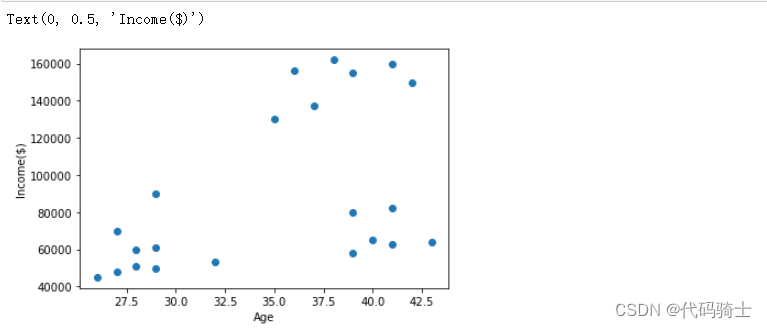
km = KMeans(n_clusters=3)#自定义选取k值为3(k值表示“簇数”、“集群数”)
y_predicted = km.fit_predict(df[['Age','Income($)']])
y_predictedarray([2, 2, 0, 0, 1, 1, 1, 1, 1, 1, 1, 0, 0, 0, 0, 0, 0, 0, 0, 2, 2, 0])
df['cluster']=y_predicted
df 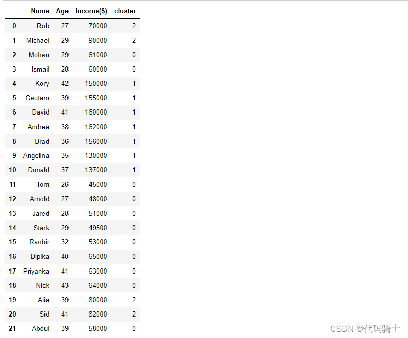
km.cluster_centers_array([[3.29090909e+01, 5.61363636e+04],
[3.82857143e+01, 1.50000000e+05],
[3.40000000e+01, 8.05000000e+04]])
df1 = df[df.cluster==0]
df2 = df[df.cluster==1]
df3 = df[df.cluster==2]
plt.scatter(df1.Age,df1['Income($)'],color='green')
plt.scatter(df2.Age,df2['Income($)'],color='red')
plt.scatter(df3.Age,df3['Income($)'],color='black')
plt.scatter(km.cluster_centers_[:,0],km.cluster_centers_[:,1],color='purple',marker='*',label='centroid')
plt.legend()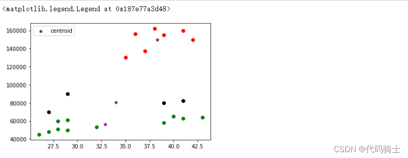
由图可见,本次聚类效果一般,因为数据集没有进行标准化。
Preprocessing using min max scaler
scaler = MinMaxScaler()
scaler.fit(df[['Income($)']])
df['Income($)'] = scaler.transform(df[['Income($)']])
scaler.fit(df[['Age']])
df['Age'] = scaler.transform(df[['Age']])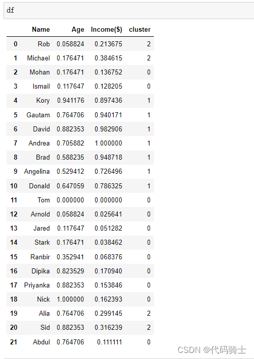
MinMaxScaler和StandardScaler的区别:
都是常见的数据预处理技术,它们的目的都是为了将数据进行缩放,以便更好地适应机器学习算法的要求。然而,这两种方法在处理数据的方式和应用场景上存在一些区别。
StandardScaler主要是通过对每个特征减去其均值并除以其标准差,将数据转换为均值为0,标准差为1的标准正态分布。因此,它经常被用于那些基于正态分布的算法,如线性回归、逻辑回归等。此外,当需要使用距离来度量相似性时,例如在使用PCA技术进行降维时,或者数据的分布不符合正态分布、存在异常值的情况下,StandardScaler往往能够提供更好的效果。
相比之下,MinMaxScaler则是通过将每个特征的最小值映射到0,最大值映射到1,然后按比例缩放其它值,使它们落于0和1之间。这种缩放技术可以帮助处理不同范围和单位的特征,进而提高模型的性能。它在不涉及距离度量、梯度、协方差计算以及数据需要被压缩到特定区间时使用广泛,比如数字图像处理中量化像素强度时,都会使用MinMaxScaler将数据压缩于[0,1]区间之中。
总的来说,选择使用哪种缩放方法主要取决于数据的分布特性以及所使用的机器学习算法的要求。
plt.scatter(df.Age,df['Income($)']) 
km = KMeans(n_clusters=3)
y_predicted = km.fit_predict(df[['Age','Income($)']])
y_predictedarray([1, 1, 1, 1, 2, 2, 2, 2, 2, 2, 2, 1, 1, 1, 1, 1, 0, 0, 0, 0, 0, 0])
df['cluster']=y_predicted
df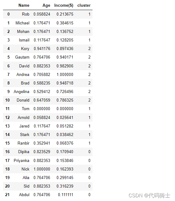
km.cluster_centers_array([[0.85294118, 0.2022792 ],
[0.1372549 , 0.11633428],
[0.72268908, 0.8974359 ]])
df1 = df[df.cluster==0]
df2 = df[df.cluster==1]
df3 = df[df.cluster==2]
plt.scatter(df1.Age,df1['Income($)'],color='green')
plt.scatter(df2.Age,df2['Income($)'],color='red')
plt.scatter(df3.Age,df3['Income($)'],color='blue')
plt.scatter(km.cluster_centers_[:,0],km.cluster_centers_[:,1],color='purple',marker='*',label='centroid')
plt.xlabel('Age')
plt.ylabel('Income ($)')
plt.legend()
Elbow Plot
Error Sum of Squares (SSE)
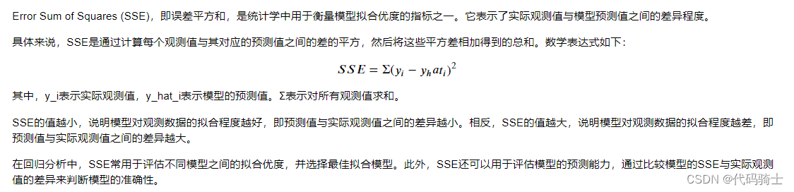
sse = []
k_rng = range(1,10)
for k in k_rng:
km = KMeans(n_clusters=k)
km.fit(df[['Age','Income($)']])
sse.append(km.inertia_)plt.xlabel('K')
plt.ylabel('Sum of squared error')
plt.plot(k_rng,sse) 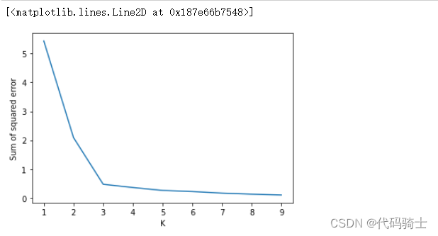
为什么选取Elbow Plot的突变点作为K?
解析:Elbow Method是一种常见的确定K值的方法,它通过绘制k值范围的平方和来选择最佳的K值。具体来说,我们计算不同K值下的聚类效果,然后以不同的K值为横坐标,簇内距离为纵坐标进行可视化。当K值由小变大的过程中,随着K值的增大簇内距离便会逐步减小,但是当K值取得最优解后簇内距离便不会出现明显的降幅。此时可以想象这么一个场景,假设某数据集以不同的K值进行聚类处理并同时计算得到对应的簇内距离和,再以不同的K值为横坐标,簇内距离为纵坐标进行可视化,便可以得到一个肘部图。在这个图中,肘部的位置就是最佳的K值。
答案: K值的选择是基于Elbow Method,该方法通过绘制k值范围的平方和来选择最佳的K值。在Elbow图中,肘部的位置就是最佳的K值。
P28-Hierarchical Clustering哪些存量客户是新产品的目标用户
https://www.youtube.com/watch?v=fjYr-76BjCw&list=PLGkfh2EpdoKU3OssXkTl3y7c9tw7jjvHm&index=26
Hierarchical Clustering(层次聚类)是一种聚类分析方法,它将数据点分组成若干个层次结构,每个层次结构内部的数据点相互之间距离较近,而不同层次结构之间的数据点距离较远。这种方法通常用于探索性数据分析和无监督学习中,可以发现数据中的模式和结构。
具体来说,Hierarchical Clustering的过程如下:
1. 首先,将每个数据点看作一个单独的簇,共有n个簇。
2. 然后,选择两个最近的簇进行合并,形成一个更大的簇。这个新的簇与原来的两个簇之间的距离最小。
3. 重复步骤2,直到所有的数据点都被合并到一个簇中。
在这个过程中,可以使用不同的距离度量方法来计算数据点之间的距离,例如欧几里得距离、曼哈顿距离等。此外,还可以使用不同的链接方式来定义簇之间的关系,例如单链接、全链接、平均链接等。
Hierarchical Clustering的结果通常以树状图的形式呈现,称为聚类树或层次结构图。从图中可以看出不同层次结构之间的关系和距离,以及每个层次结构内部的数据点的相似度。
from IPython.display import Image
Image(filename='C:\\Users\86185\Desktop\\TempDesktop\\研究内容\\Python学习\\Py机深文字教程+源码\\LessonPythonCode-main\\Lesson28-Dendrogram.png')
#C:\Users\86185\Desktop\TempDesktop\研究内容\Python学习\Py机深文字教程+源码\LessonPythonCode-main

from IPython.display import Image
Image(filename='C:\\Users\86185\Desktop\\TempDesktop\\研究内容\\Python学习\\Py机深文字教程+源码\\LessonPythonCode-main\\Lesson28-Clustering_h1.png')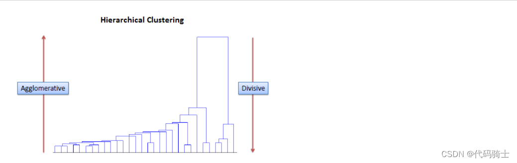
import pandas as pd
import numpy as np
import matplotlib.pyplot as plt
%matplotlib inlinedata = pd.read_csv('Lesson28-customers data.csv')
data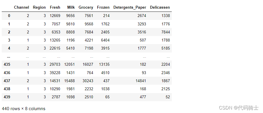
data.describe()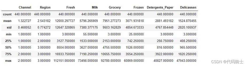
data.info()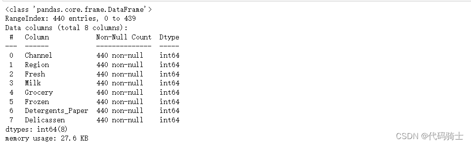
data.isnull().sum()
data['Channel'].unique()array([2, 1], dtype=int64)
data['Region'].unique()array([3, 1, 2], dtype=int64)

数据标准化的几种不同方式
from sklearn.preprocessing import StandardScaler
sc=StandardScaler()
scaled_data=sc.fit_transform(data)from sklearn.preprocessing import normalize
norm_data=normalize(data)StandardScaler standardizes features by removing the mean and scaling to unit variance, Normalizer rescales each sample. The main difference is that Standard Scalar is applied on Columns, while Normalizer is applied on rows, So make sure you reshape your data before normalizing it
StandardScaler通过去除均值和缩放到单位方差来标准化特征,Normalizer重新调整每个样本。主要区别在于Standard Scalar应用于列,而Normalizer应用于行,因此在标准化之前请确保您已将数据重塑为正确的形状。
from IPython.display import Image
Image(filename='C:\\Users\86185\Desktop\\TempDesktop\\研究内容\\Python学习\\Py机深文字教程+源码\\LessonPythonCode-main\\Lesson28-scaling.png')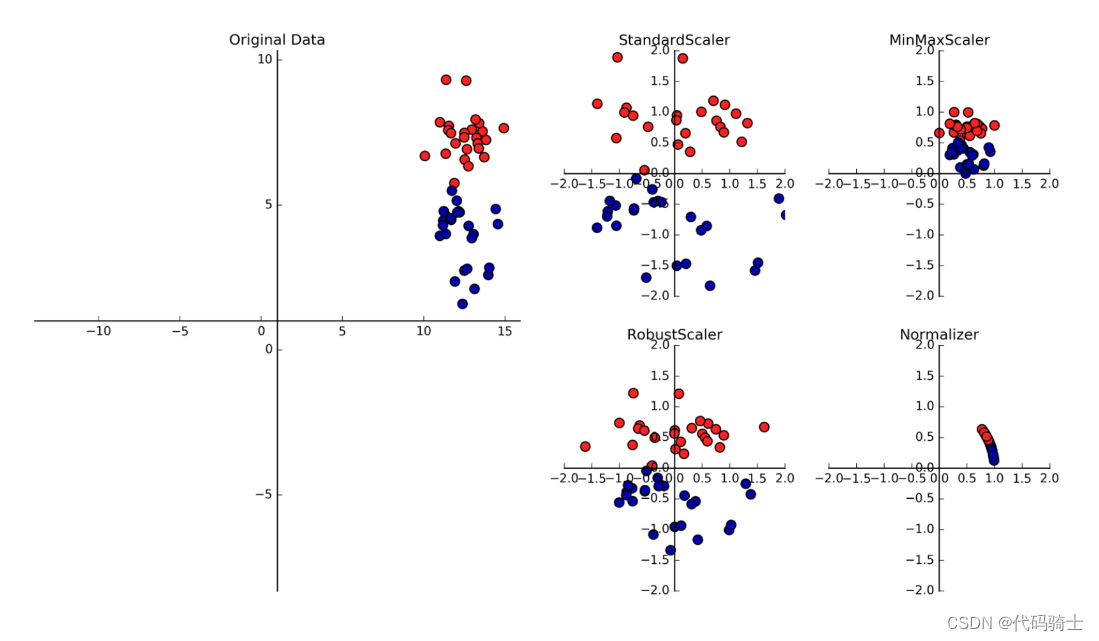
df=pd.DataFrame(scaled_data,columns=data.columns)
df1=pd.DataFrame(norm_data,columns=data.columns)
import scipy.cluster.hierarchy as shc
plt.figure(figsize=[10,7])
plt.title('Dendrogram')
dend=shc.dendrogram(shc.linkage(df,method='ward'))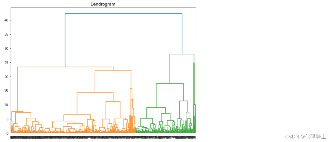
import scipy.cluster.hierarchy as shc
plt.figure(figsize=[10,7])
plt.title('Dendrogram')
dend=shc.dendrogram(shc.linkage(df1,method='ward'))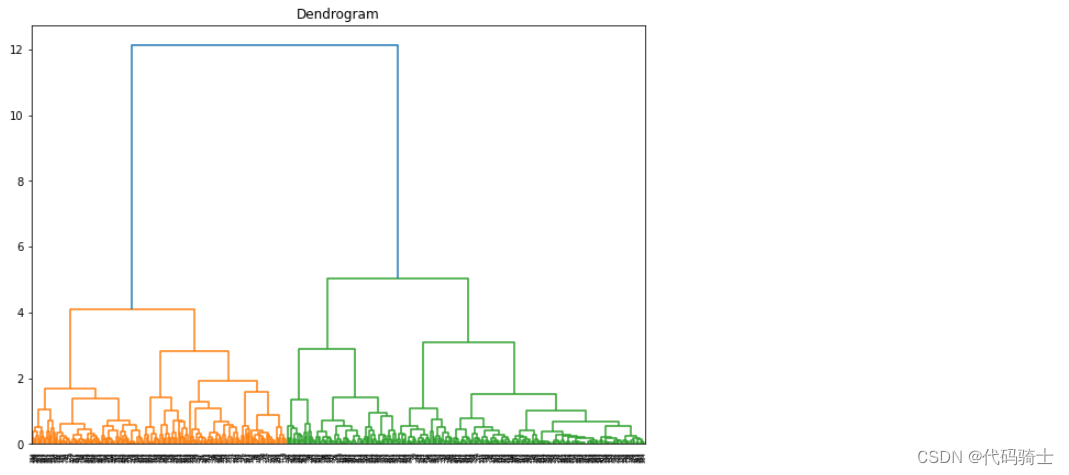
import scipy.cluster.hierarchy as shc
plt.figure(figsize=[10,7])
plt.title('Dendrogram')
dend=shc.dendrogram(shc.linkage(df,method='single'))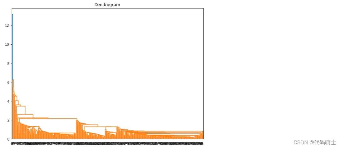
import scipy.cluster.hierarchy as shc
plt.figure(figsize=[10,7])
plt.title('Dendrogram')
dend=shc.dendrogram(shc.linkage(df,method='complete'))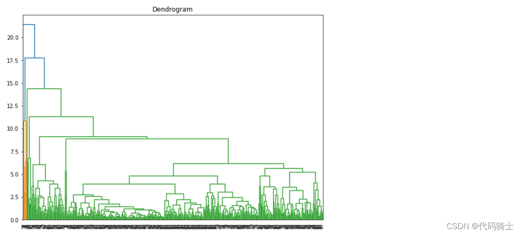
import scipy.cluster.hierarchy as shc
plt.figure(figsize=[10,7])
plt.title('Dendrogram')
dend=shc.dendrogram(shc.linkage(df,method='average'))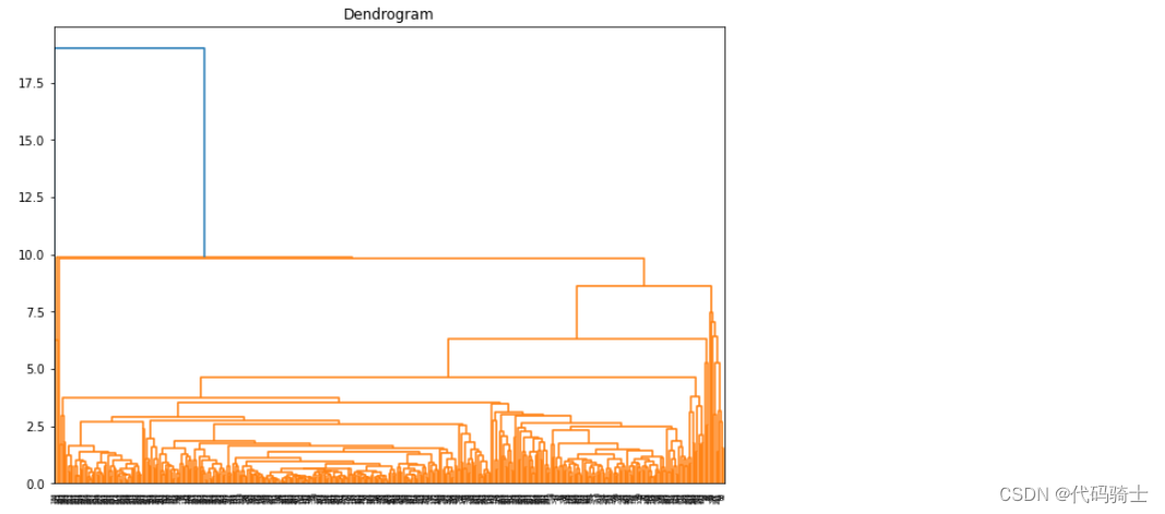
plt.figure(figsize=(10, 7))
plt.title("Dendrograms")
dend = shc.dendrogram(shc.linkage(df1, method='ward'))
plt.axhline(y=6, color='r', linestyle='--')
from sklearn.cluster import AgglomerativeClustering
cluster=AgglomerativeClustering(n_clusters=2,affinity='euclidean',linkage='ward')
cluster.fit_predict(df1)array([1, 1, 1, 0, 0, 1, 0, 1, 1, 1, 1, 0, 0, 0, 0, 0, 1, 1, 0, 0, 0, 0,
0, 1, 0, 0, 0, 0, 1, 0, 0, 1, 0, 0, 1, 1, 0, 1, 1, 0, 0, 0, 1, 1,
1, 1, 1, 1, 1, 1, 0, 1, 0, 1, 0, 1, 1, 1, 0, 1, 0, 1, 1, 1, 0, 1,
1, 0, 1, 0, 0, 0, 0, 0, 1, 0, 0, 1, 0, 1, 0, 1, 1, 0, 0, 1, 1, 0,
0, 0, 0, 0, 1, 0, 1, 1, 1, 0, 0, 0, 1, 1, 1, 0, 0, 0, 1, 1, 1, 1,
0, 1, 0, 0, 0, 0, 0, 1, 0, 0, 0, 0, 0, 1, 0, 0, 0, 0, 1, 0, 0, 0,
0, 0, 0, 0, 1, 1, 0, 1, 0, 0, 0, 0, 0, 1, 0, 0, 0, 0, 0, 1, 0, 1,
0, 1, 1, 0, 1, 1, 1, 0, 0, 1, 1, 1, 1, 1, 0, 0, 1, 1, 1, 1, 1, 1,
0, 0, 0, 1, 0, 0, 1, 1, 1, 0, 0, 1, 1, 1, 0, 0, 0, 1, 0, 0, 0, 1,
0, 0, 1, 1, 0, 1, 1, 1, 0, 1, 1, 1, 0, 1, 0, 1, 1, 1, 1, 0, 1, 0,
0, 1, 0, 0, 0, 0, 0, 0, 1, 0, 0, 1, 0, 1, 0, 1, 0, 0, 0, 0, 0, 0,
0, 0, 1, 1, 0, 0, 0, 0, 0, 1, 0, 0, 1, 0, 0, 0, 0, 0, 0, 0, 0, 1,
1, 1, 1, 0, 1, 0, 0, 1, 1, 0, 1, 1, 0, 0, 0, 0, 1, 0, 0, 0, 0, 0,
0, 0, 0, 0, 1, 0, 1, 1, 0, 0, 0, 0, 1, 1, 0, 1, 1, 1, 1, 1, 1, 0,
0, 1, 0, 0, 1, 0, 0, 1, 0, 1, 0, 1, 1, 0, 0, 0, 0, 0, 0, 1, 0, 0,
0, 1, 0, 1, 0, 0, 0, 0, 0, 0, 1, 1, 1, 1, 0, 1, 1, 0, 1, 1, 0, 1,
1, 1, 0, 1, 0, 1, 1, 1, 0, 0, 1, 0, 0, 1, 0, 0, 0, 0, 0, 0, 1, 0,
0, 0, 1, 0, 1, 1, 0, 0, 0, 0, 1, 0, 1, 0, 0, 0, 0, 1, 1, 0, 0, 0,
1, 0, 0, 0, 0, 0, 0, 0, 0, 0, 0, 1, 0, 0, 0, 1, 1, 0, 0, 1, 1, 1,
1, 0, 1, 0, 0, 0, 0, 0, 1, 0, 1, 0, 1, 0, 0, 1, 0, 0, 0, 1, 0, 1],
dtype=int64)
df1['cluster']=cluster.fit_predict(df1)
cluster.labels_array([1, 1, 1, 0, 0, 1, 0, 1, 1, 1, 1, 0, 0, 0, 0, 0, 1, 1, 0, 0, 0, 0,
0, 1, 0, 0, 0, 0, 1, 0, 0, 1, 0, 0, 1, 1, 0, 1, 1, 0, 0, 0, 1, 1,
1, 1, 1, 1, 1, 1, 0, 1, 0, 1, 0, 1, 1, 1, 0, 1, 0, 1, 1, 1, 0, 1,
1, 0, 1, 0, 0, 0, 0, 0, 1, 0, 0, 1, 0, 1, 0, 1, 1, 0, 0, 1, 1, 0,
0, 0, 0, 0, 1, 0, 1, 1, 1, 0, 0, 0, 1, 1, 1, 0, 0, 0, 1, 1, 1, 1,
0, 1, 0, 0, 0, 0, 0, 1, 0, 0, 0, 0, 0, 1, 0, 0, 0, 0, 1, 0, 0, 0,
0, 0, 0, 0, 1, 1, 0, 1, 0, 0, 0, 0, 0, 1, 0, 0, 0, 0, 0, 1, 0, 1,
0, 1, 1, 0, 1, 1, 1, 0, 0, 1, 1, 1, 1, 1, 0, 0, 1, 1, 1, 1, 1, 1,
0, 0, 0, 1, 0, 0, 1, 1, 1, 0, 0, 1, 1, 1, 0, 0, 0, 1, 0, 0, 0, 1,
0, 0, 1, 1, 0, 1, 1, 1, 0, 1, 1, 1, 0, 1, 0, 1, 1, 1, 1, 0, 1, 0,
0, 1, 0, 0, 0, 0, 0, 0, 1, 0, 0, 1, 0, 1, 0, 1, 0, 0, 0, 0, 0, 0,
0, 0, 1, 1, 0, 0, 0, 0, 0, 1, 0, 0, 1, 0, 0, 0, 0, 0, 0, 0, 0, 1,
1, 1, 1, 0, 1, 0, 0, 1, 1, 0, 1, 1, 0, 0, 0, 0, 1, 0, 0, 0, 0, 0,
0, 0, 0, 0, 1, 0, 1, 1, 0, 0, 0, 0, 1, 1, 0, 1, 1, 1, 1, 1, 1, 0,
0, 1, 0, 0, 1, 0, 0, 1, 0, 1, 0, 1, 1, 0, 0, 0, 0, 0, 0, 1, 0, 0,
0, 1, 0, 1, 0, 0, 0, 0, 0, 0, 1, 1, 1, 1, 0, 1, 1, 0, 1, 1, 0, 1,
1, 1, 0, 1, 0, 1, 1, 1, 0, 0, 1, 0, 0, 1, 0, 0, 0, 0, 0, 0, 1, 0,
0, 0, 1, 0, 1, 1, 0, 0, 0, 0, 1, 0, 1, 0, 0, 0, 0, 1, 1, 0, 0, 0,
1, 0, 0, 0, 0, 0, 0, 0, 0, 0, 0, 1, 0, 0, 0, 1, 1, 0, 0, 1, 1, 1,
1, 0, 1, 0, 0, 0, 0, 0, 1, 0, 1, 0, 1, 0, 0, 1, 0, 0, 0, 1, 0, 1],
dtype=int64)
plt.figure(figsize=[10,7])
plt.scatter(df1.Milk,df1.Grocery,c=cluster.labels_)
plt.figure(figsize=(10, 7))
plt.scatter(df1['Milk'], df1['Fresh'], c=cluster.labels_) 
P29-DBSCAN聚类(基于密度的空间聚类应用噪声)与K means(K均值)及Hierarchical Clustering(层次聚类)区别
https://www.youtube.com/watch?v=XamM0h4r0Qo&list=PLGkfh2EpdoKU3OssXkTl3y7c9tw7jjvHm&index=27
DBSCAN、K-means和Hierarchical Clustering是三种常用的数据聚类算法,它们在处理数据的方式上存在显著的差异。
1. **基于方法的区别**:
- **DBSCAN (Density-Based Spatial Clustering of Applications with Noise)**:这是一种基于密度的聚类算法,它可以识别出数据集中的噪声点并有效地处理它们。与K-means不同,DBSCAN不需要预先指定聚类的簇数。其核心思想是将密度相连的数据点组合在一起形成簇。
- **K-means**:这是一种基于距离的聚类算法,它将距离相近的数据点视为相似的点并将它们归为一类。K-means需要用户预先指定聚类的簇数,并且初始聚类中心的选择对最终的聚类结果有很大的影响。
- **Hierarchical Clustering**:这是一种基于树的方法,它在不同层次上对数据集进行划分,从而形成树状的聚类结构。与其他两种方法不同,层次聚类可以为用户提供一个层次性的聚类结果,而不是仅仅提供一个硬性的聚类标签。2. **处理异常值的能力**:
- **DBSCAN**:能够有效地处理数据集中的噪声点和异常值。
- **K-means**:对于噪声点和异常值较为敏感,这些值可能会影响最终的聚类结果。3. **形态假设**:
- **K-means**:假定所有的簇都是球形的,这可能不适用于所有类型的数据集。
- **DBSCAN**:没有关于数据形态的假设,因此可以对任意形状的簇进行聚类。
from IPython.display import Image
Image(filename='C:\\Users\\86185\\Desktop\\TempDesktop\\研究内容\\Python学习\\Py机深文字教程+源码\\LessonPythonCode-main\\Lesson29-Demo.gif')
#C:\Users\86185\Desktop\TempDesktop\研究内容\Python学习\Py机深文字教程+源码\LessonPythonCode-main 
基于密度的空间聚类应用噪声(DBSCAN)
DBSCAN是一种用于机器学习的聚类方法,用于将高密度簇与低密度簇分开。由于DBSCAN是基于密度的聚类算法,因此它非常适合在数据中寻找具有高观测密度的区域,相对于数据中不太密集的区域。DBSCAN还可以将数据分类为不同形状的簇,这是另一个强大的优势。
DBSCAN的优点:- 在给定的数据集中,擅长将高密度簇与低密度簇分开。- 擅长处理数据集中的异常值。
DBSCAN的缺点:- 虽然DBSCAN擅长将高密度簇与低密度簇分开,但对于相似密度的簇却很困难。- 难以处理高维数据。
minPts:考虑一个区域为密集所需的最小点数(阈值)。
eps(ε):用于定位任何点周围点的的距离度量。
from IPython.display import Image
Image(filename='C:\\Users\\86185\\Desktop\\TempDesktop\\研究内容\\Python学习\\Py机深文字教程+源码\\LessonPythonCode-main\\Lesson29-Clustering1.png') 
from IPython.display import Image
Image(filename='C:\\Users\\86185\\Desktop\\TempDesktop\\研究内容\\Python学习\\Py机深文字教程+源码\\LessonPythonCode-main\\Lesson29-DBSCAN-1.png')
from IPython.display import Image
Image(filename='D:\\python\\Project0-Python-MachineLearning\\Lesson29-DBSCAN.png')
from IPython.display import Image
Image(filename='C:\\Users\\86185\\Desktop\\TempDesktop\\研究内容\\Python学习\\Py机深文字教程+源码\\LessonPythonCode-main\\Lesson29-DBSCAN-2.png') 
#DBSCAN with cluster spherical data
import numpy as np
from sklearn.cluster import DBSCAN
from sklearn import metrics
from sklearn.datasets import make_blobs
from sklearn.preprocessing import StandardScaler
# Generate sample data
centers = [[1, 1], [-1, -1], [1, -1]]
X, labels_true = make_blobs(n_samples=750, centers=centers, cluster_std=0.4,
random_state=0) 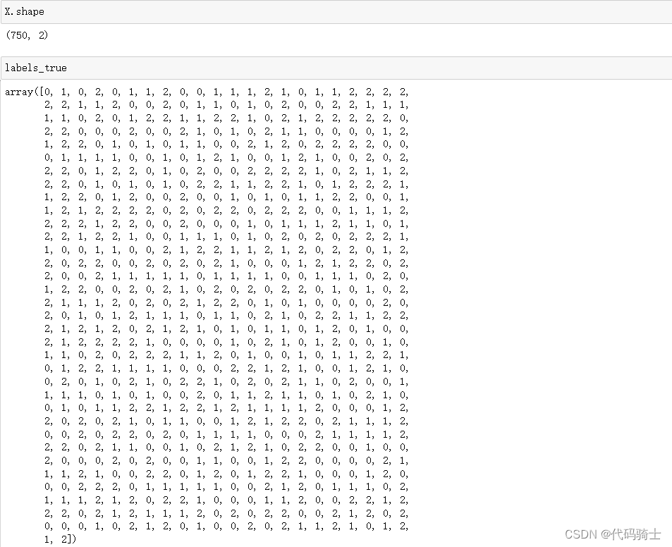
X = StandardScaler().fit_transform(X)#表示将标准尺度下的X数据转换为标准化向量。
# Compute DBSCAN
db = DBSCAN(eps=0.3, min_samples=10).fit(X)
core_samples_mask = np.zeros_like(db.labels_, dtype=bool)
core_samples_mask[db.core_sample_indices_] = True
labels = db.labels_ 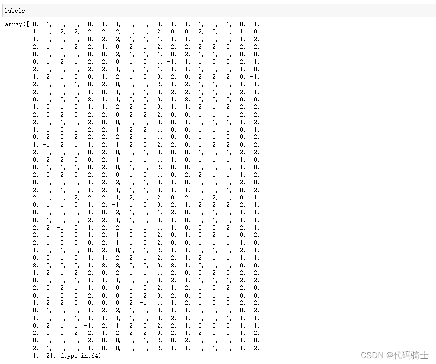
# Number of clusters in labels, ignoring noise if present.
n_clusters_ = len(set(labels)) - (1 if -1 in labels else 0)
n_noise_ = list(labels).count(-1) 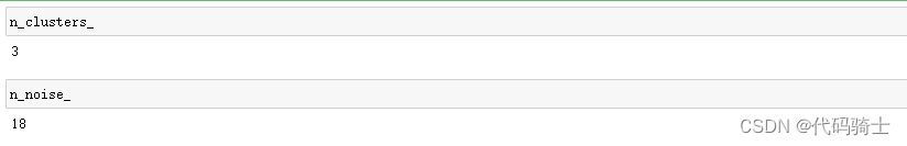
print('Estimated number of clusters: %d' % n_clusters_)
print('Estimated number of noise points: %d' % n_noise_)
print("Homogeneity: %0.3f" % metrics.homogeneity_score(labels_true, labels))
print("Completeness: %0.3f" % metrics.completeness_score(labels_true, labels))
print("V-measure: %0.3f" % metrics.v_measure_score(labels_true, labels))
print("Adjusted Rand Index: %0.3f"
% metrics.adjusted_rand_score(labels_true, labels))
print("Adjusted Mutual Information: %0.3f"
% metrics.adjusted_mutual_info_score(labels_true, labels))
print("Silhouette Coefficient: %0.3f"
% metrics.silhouette_score(X, labels))Estimated number of clusters: 3 Estimated number of noise points: 18 Homogeneity: 0.953 Completeness: 0.883 V-measure: 0.917 Adjusted Rand Index: 0.952 Adjusted Mutual Information: 0.916 Silhouette Coefficient: 0.626
# Plot result
import matplotlib.pyplot as plt
%matplotlib inline
# Black removed and is used for noise instead.
unique_labels = set(labels) 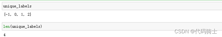
colors = [plt.cm.Spectral(each)
for each in np.linspace(0, 1, len(unique_labels))] 
for k, col in zip(unique_labels, colors):
if k == -1:
# Black used for noise.
col = [0, 0, 0, 1]
class_member_mask = (labels == k)
xy = X[class_member_mask & core_samples_mask]
plt.plot(xy[:, 0], xy[:, 1], 'o', markerfacecolor=tuple(col),
markeredgecolor='k', markersize=14)
xy = X[class_member_mask & ~core_samples_mask]
plt.plot(xy[:, 0], xy[:, 1], 'o', markerfacecolor=tuple(col),
markeredgecolor='k', markersize=6)
plt.title('Estimated number of clusters: %d' % n_clusters_)
plt.show() 
#DBSCAN to cluster circle data
import numpy as np
import matplotlib.pyplot as plt
from sklearn import metrics
from sklearn.datasets import make_circles
from sklearn.preprocessing import StandardScaler
from sklearn.cluster import DBSCAN
X, y = make_circles(n_samples=750, factor=0.3, noise=0.1)
X = StandardScaler().fit_transform(X)
y_pred = DBSCAN(eps=0.3, min_samples=10).fit_predict(X)
plt.scatter(X[:,0], X[:,1], c=y_pred)
print('Number of clusters: {}'.format(len(set(y_pred[np.where(y_pred != -1)]))))
print('Homogeneity: {}'.format(metrics.homogeneity_score(y, y_pred)))
print('Completeness: {}'.format(metrics.completeness_score(y, y_pred)))
print("V-measure: %0.3f" % metrics.v_measure_score(labels_true, labels))
print("Adjusted Rand Index: %0.3f"
% metrics.adjusted_rand_score(labels_true, labels))
print("Adjusted Mutual Information: %0.3f"
% metrics.adjusted_mutual_info_score(labels_true, labels))
print("Silhouette Coefficient: %0.3f"
% metrics.silhouette_score(X, labels))Number of clusters: 2 Homogeneity: 1.0 Completeness: 0.9514032557784387 V-measure: 0.917 Adjusted Rand Index: 0.952 Adjusted Mutual Information: 0.916 Silhouette Coefficient: -0.031
from IPython.display import Image
Image(filename='C:\\Users\\86185\\Desktop\\TempDesktop\\研究内容\\Python学习\\Py机深文字教程+源码\\LessonPythonCode-main\Lesson29-Kmeans.png') 
P30-纽约Uber数据分析图形化和K means计算热点
https://www.youtube.com/watch?v=gT7w7Ex_72s&list=PLGkfh2EpdoKU3OssXkTl3y7c9tw7jjvHm&index=28
Folium是一个Python库,用于创建交互式地图。它基于Leaflet.js,可以轻松地将地图可视化添加到Python项目中。
下载安装第三方库:
pip install folium
import numpy as np # linear algebra
import pandas as pd # data processing, CSV file I/O (e.g. pd.read_csv)
import matplotlib.pyplot as plt
import seaborn as sns
import folium #visualize map
from sklearn.cluster import KMeans #k-means clustering
from yellowbrick.cluster import KElbowVisualizer #Elbow visualize K-means#Date/Time : The date and time of the Uber pickup
#Lat : The latitude of the Uber pickup
#Lon : The longitude of the Uber pickup
#Base : The TLC base company code affiliated with the Uber pickup
'''
B02512 : Unter
B02598 : Hinter
B02617 : Weiter
B02682 : Schmecken
B02764 : Danach-NY
B02765 : Grun
B02835 : Dreist
B02836 : Drinnen
'''
df_ori = pd.read_csv('Lesson30-uber-raw-data-aug14.csv') #from https://www.kaggle.com/
df_ori
df_ori.info()<class 'pandas.core.frame.DataFrame'> RangeIndex: 829275 entries, 0 to 829274 Data columns (total 4 columns): # Column Non-Null Count Dtype --- ------ -------------- ----- 0 Date/Time 829275 non-null object 1 Lat 829275 non-null float64 2 Lon 829275 non-null float64 3 Base 829275 non-null object dtypes: float64(2), object(2) memory usage: 25.3+ MB
df_ori['Base'].unique()array(['B02512', 'B02598', 'B02617', 'B02682', 'B02764'], dtype=object)
from IPython.display import Image
#C:\Users\86185\Desktop\TempDesktop\研究内容\Python学习\Py机深文字教程+源码\LessonPythonCode-main
Image(filename='C:\\Users\\86185\\Desktop\\TempDesktop\\研究内容\\Python学习\\Py机深文字教程+源码\\LessonPythonCode-main\\Lesson30-B02512.png')
from IPython.display import Image
Image(filename='C:\\Users\\86185\\Desktop\\TempDesktop\\研究内容\\Python学习\\Py机深文字教程+源码\\LessonPythonCode-main\\Lesson30-B02617.png') 
clus_k_ori = df_ori[['Lat', 'Lon']]
clus_k_ori.dtypesLat float64 Lon float64 dtype: object
import time
start = time.time()
import matplotlib.pyplot as plt
from sklearn.cluster import KMeans
from yellowbrick.cluster import KElbowVisualizer
model_ori = KMeans()
visualizer = KElbowVisualizer(model_ori, k = (1, 18)) #k = 1 to 17
visualizer.fit(clus_k_ori)
visualizer.show()
time2=time
end = time.time()
end-start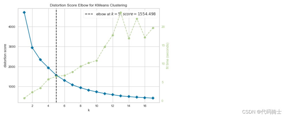
196.65676426887512
kmeans_ori = KMeans(n_clusters = 5, random_state = 0) #k = 5
kmeans_ori.fit(clus_k_ori)KMeans(n_clusters=5, random_state=0)
centroids_k_ori = kmeans_ori.cluster_centers_
centroids_k_oriarray([[ 40.75813164, -73.98089683],
[ 40.70819256, -73.98534917],
[ 40.66869811, -73.75817069],
[ 40.79725343, -73.88727189],
[ 40.6961372 , -74.19972869]])
clocation_k_ori = pd.DataFrame(centroids_k_ori, columns = ['Latitude', 'Longitude'])clocation_k_ori
plt.scatter(clocation_k_ori['Latitude'], clocation_k_ori['Longitude'], marker = "x", color = 'r', s = 200)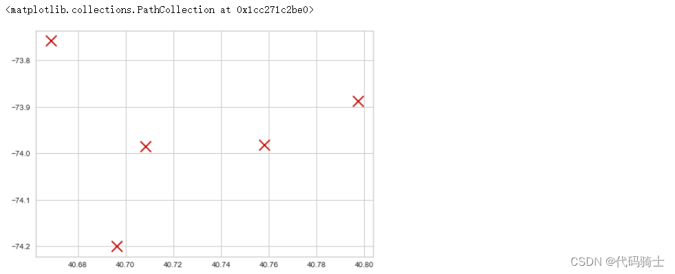
clocation_k_ori.values.tolist()[[40.75813163909047, -73.98089683164005], [40.70819255961724, -73.98534916648876], [40.66869811488646, -73.75817068846192], [40.79725342625452, -73.88727189048329], [40.69613720447469, -74.19972869334563]]
centroid_k_ori[0][40.66869811488647, -73.75817068846192]
centroid_k_ori = clocation_k_ori.values.tolist()
map_k_ori = folium.Map(location = [40.71600413400166, -73.98971408426613], zoom_start = 10)
for point in range(0, len(centroid_k_ori)):
folium.Marker(centroid_k_ori[point], popup = centroid_k_ori[point]).add_to(map_k_ori)
map_k_ori
Make this Notebook Trusted to load map: File -> Trust Notebook

label_k_ori = kmeans_ori.labels_
label_k_oriarray([3, 1, 1, ..., 3, 3, 1])
df_new_k = df_ori.copy()
df_new_k['Clusters'] = label_k_ori
df_new_k
sns.catplot(data = df_new_k, x = "Clusters", kind = "count", height = 7, aspect = 2)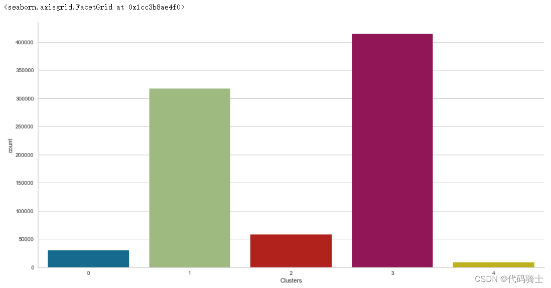
count_3 = 0
count_0 = 0
for value in df_new_k['Clusters']:
if value == 3:
count_3 += 1
if value == 0:
count_0 += 1
print(count_0, count_3)30346 414279
new_location_ori = [(40.76, -73.99)]
kmeans_ori.predict(new_location_ori)array([0])
kmeans_ori.predict(new_location_ori)array([0])
new_location_ori = [40.76, -74.1]
map_k_ori = folium.Map(location = [40.71600413400166, -73.98971408426613], zoom_start = 10)
folium.Marker(new_location_ori, popup = new_location_ori).add_to(map_k_ori)
map_k_ori
df_ori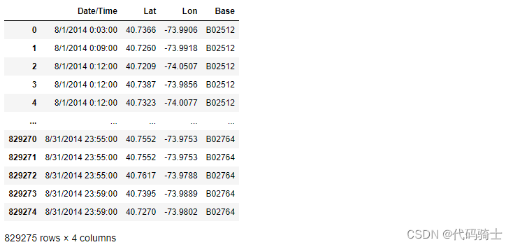
df_ori.columns = ['timestamp', 'lat', 'lon', 'base']
df_ori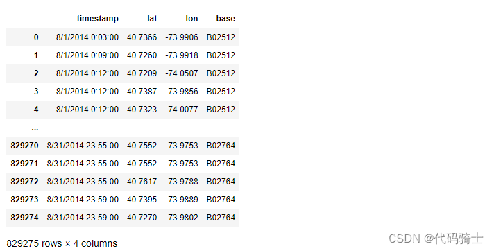
import time
ti = time.time()
df_ori['timestamp'] = pd.to_datetime(df_ori['timestamp'])
tf = time.time()
print(tf-ti,' seconds.')60.2118775844574 seconds.
df_ori 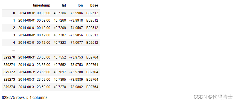
df_ori['weekday'] = df_ori.timestamp.dt.weekday
df_ori['month'] = df_ori.timestamp.dt.month
df_ori['day'] = df_ori.timestamp.dt.day
df_ori['hour'] = df_ori.timestamp.dt.hour
df_ori['minute'] = df_ori.timestamp.dt.minutedf_ori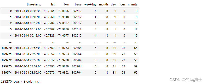
## Hourly Ride Data
## groupby operation
hourly_ride_data = df_ori.groupby(['day','hour','weekday'])['timestamp'].count()
## reset index
hourly_ride_data = hourly_ride_data.reset_index()
## rename column
hourly_ride_data = hourly_ride_data.rename(columns = {'timestamp':'ride_count'})
## ocular analysis
hourly_ride_data 
## Weekday Hourly Averages
## groupby operation
weekday_hourly_avg = hourly_ride_data.groupby(['weekday','hour'])['ride_count'].mean()
## reset index
weekday_hourly_avg = weekday_hourly_avg.reset_index()
## rename column
weekday_hourly_avg = weekday_hourly_avg.rename(columns = {'ride_count':'average_rides'})
## sort by categorical index
weekday_hourly_avg = weekday_hourly_avg.sort_index()
## ocular analysis
weekday_hourly_avg
##Define Color Palette
tableau_color_blind = [(0, 107, 164), (255, 128, 14), (171, 171, 171), (89, 89, 89),
(95, 158, 209), (200, 82, 0), (137, 137, 137), (163, 200, 236),
(255, 188, 121), (207, 207, 207)]
for i in range(len(tableau_color_blind)):
r, g, b = tableau_color_blind[i]
tableau_color_blind[i] = (r / 255., g / 255., b / 255.)## create figure
fig = plt.figure(figsize=(12,6))
ax = fig.add_subplot(111)
## set palette
current_palette = sns.color_palette(tableau_color_blind)
## plot data
sns.pointplot(ax=ax, x='hour',y='average_rides',hue='weekday',
palette = current_palette, data = weekday_hourly_avg)
## clean up the legend
l = ax.legend()
l.set_title('')
## format plot labels
ax.set_title('Weekday Averages for August 2014', fontsize=30)
ax.set_ylabel('Rides per Hour', fontsize=20)
ax.set_xlabel('Hour', fontsize=20)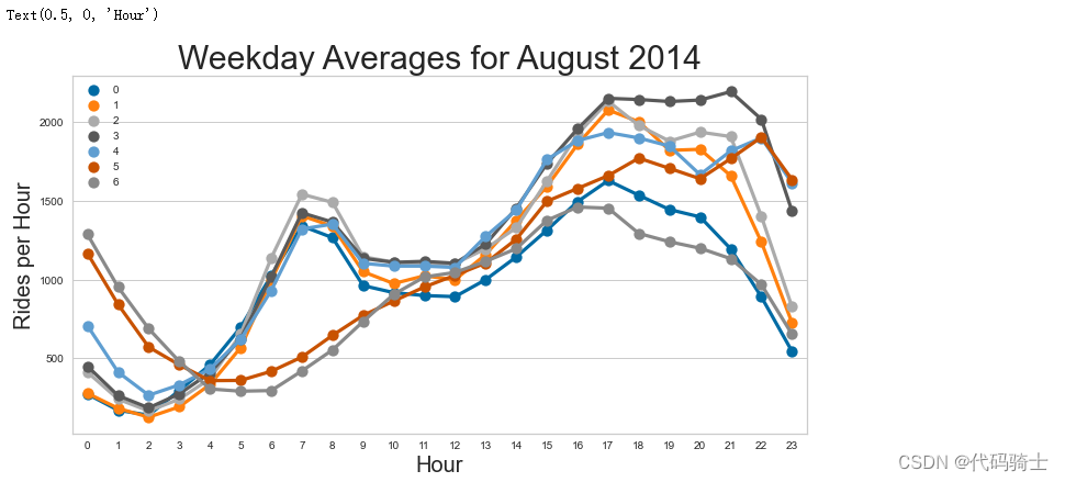
%matplotlib inline
plt.figure(figsize=(16, 12))
plt.plot(df_ori.lon, df_ori.lat, '.', ms=.8, alpha=.5)
plt.ylim(bottom=40.5,top=41)
plt.xlim(left=-74.4,right=-73.5)
plt.xlabel('Longitude')
plt.ylabel('Latitude')
plt.title('New York Uber Pickups 2014')
plt.show()
from folium.plugins import HeatMap
lat_lon = df_ori[["lat", "lon"]].values[:10000]
uber_map = folium.Map(location=[40.7128, -74.0060], zoom_start=12)
#A heatmap can be plotted like so... the radius argument controls the radius of each point within the map
#You can zoom in on this map to see more specific areas, or out to see more general
HeatMap(lat_lon, fradius=13).add_to(uber_map)
uber_map
P31-KMeans clustering如何验证K点最佳 silhouette analysis
https://www.youtube.com/watch?v=UxcAcyQ7DZE&list=PLGkfh2EpdoKU3OssXkTl3y7c9tw7jjvHm&index=31
KMeans聚类算法是一种常用的无监督学习算法,用于将数据集划分为K个不同的簇。在实际应用中,我们通常需要确定最佳的K值,以便获得最佳的聚类效果。
Silhouette Analysis(轮廓分析)是一种常用的评估聚类效果的方法,它通过计算每个样本的轮廓系数来评估聚类结果的好坏。轮廓系数是一个介于-1和1之间的值,越接近1表示样本与其所在簇内的其他样本越相似,而与其他簇的样本差异越大;越接近-1表示样本与其所在簇内的其他样本差异越大,而与其他簇的样本越相似。
为了验证K点最佳,我们可以使用Silhouette Analysis方法对不同K值下的聚类结果进行评估,并选择具有最大平均轮廓系数的K值作为最佳K值。具体步骤如下:
1. 对于给定的数据集,使用KMeans算法分别对不同K值(例如K=2,3,4...)进行聚类。
2. 对于每个K值下的聚类结果,计算每个样本的轮廓系数。轮廓系数的计算公式为:
s(i) = (b(i) - a(i)) / max(a(i), b(i))
其中,a(i)表示样本i与其所处簇内其他样本的平均距离;b(i)表示样本i与最近簇内其他样本的平均距离。
3. 计算每个K值下所有样本的平均轮廓系数,并选择具有最大平均轮廓系数的K值作为最佳K值。
需要注意的是,Silhouette Analysis方法只能给出相对的评价结果,不能保证找到全局最优的K值。因此,在实际应用中,我们还需要结合领域知识和其他评估指标来综合判断最佳的K值。
代码演示:
from sklearn.datasets import make_blobs
from sklearn.cluster import KMeans
from sklearn.metrics import silhouette_samples, silhouette_score
import matplotlib.pyplot as plt
import matplotlib.cm as cm
import numpy as np# Generating the sample data from make_blobs
# This particular setting has one distinct cluster and 3 clusters placed close
# together.
X, y = make_blobs(n_samples=500,
n_features=2,
centers=4,
cluster_std=1,
center_box=(-10.0, 10.0),
shuffle=True,
random_state=1) # For reproducibility
from sklearn.cluster import KMeans
wcss=[]
for i in range(1,11):
kmeans=KMeans(n_clusters=i, init='k-means++',random_state=0)
kmeans.fit(X)
wcss.append(kmeans.inertia_)
plt.plot(range(1,11),wcss)
plt.title('The Elbow Method')
plt.xlabel('Number of Clusters')
plt.ylabel('WCSS')
plt.show()
使用 yellowbrick 判断最佳K值
Yellowbrick是一个用于数据探索和可视化的Python库,它提供了一些工具来帮助用户更好地理解和解释他们的机器学习模型。其中,KElbowVisualizer是Yellowbrick库中的一个类,主要用于可视化K-means聚类算法的最优聚类数(即Elbow Method)。
Elbow Method是一种确定最优K值(即聚类的数量)的方法。在这个方法中,我们试图通过将数据集划分为不同的聚类数量并计算每个聚类的误差平方和(SSE)来找到最佳的K值。随着聚类数量的增加,SSE通常会减少,但当达到某个点时,增加更多的聚类对SSE的影响会越来越小。这个“弯曲”的地方就是所谓的“肘部”,也就是我们选择最优K值的地方。
KElbowVisualizer类就是用来帮助我们找到这个“肘部”的工具。它接受一个已经训练好的KMeans模型和一个数据集作为输入,然后生成一个图形,显示了不同聚类数量下的SSE。通过观察这个图形,我们可以直观地看到何时开始过度拟合(即SSE不再显著减小),从而选择出最优的K值。
pip install yellowbrick

import matplotlib.pyplot as plt
from sklearn.cluster import KMeans
from yellowbrick.cluster import KElbowVisualizer
model_ori = KMeans()
visualizer = KElbowVisualizer(model_ori, k = (1, 11)) #k = 1 to 11
visualizer.fit(X)
visualizer.show()
clusterer = KMeans(n_clusters=4, random_state=10)
cluster_labels = clusterer.fit_predict(X)
print(cluster_labels)[2 2 0 1 3 1 3 3 3 3 2 2 3 1 3 2 3 2 1 3 0 0 3 1 3 3 1 1 0 3 2 1 3 2 3 2 0 0 2 0 3 0 1 3 3 2 0 3 1 1 1 0 0 3 2 0 0 0 0 3 1 1 0 3 1 3 2 3 0 0 2 0 3 2 3 3 2 3 3 0 1 1 0 1 1 0 0 1 0 0 1 2 0 3 1 2 2 3 2 1 1 2 1 0 1 3 3 1 1 0 3 2 1 0 1 0 1 3 1 3 0 2 2 0 3 0 1 2 2 3 1 0 0 0 0 2 1 3 1 1 3 2 3 1 1 1 3 3 2 2 0 0 1 2 1 0 0 0 0 0 0 0 0 0 1 2 2 2 3 1 2 0 3 2 1 0 0 0 0 2 3 0 1 2 2 0 3 2 2 3 1 1 2 2 3 1 3 2 2 1 2 0 1 3 3 2 3 0 2 3 0 3 0 2 3 3 3 1 0 1 3 2 0 3 0 0 0 1 0 1 2 0 2 0 1 1 0 2 1 2 3 0 2 2 2 2 3 0 2 0 3 1 1 3 3 1 0 3 0 1 3 1 0 0 1 3 2 2 0 0 0 3 1 1 3 1 0 2 1 2 1 2 2 1 2 1 1 3 0 0 0 3 3 0 2 1 2 2 2 3 0 3 2 0 2 2 0 2 2 0 1 2 3 3 1 1 0 2 1 1 3 2 1 1 3 0 1 0 3 2 2 1 0 2 3 1 1 3 3 3 2 3 1 1 0 1 1 1 1 2 2 3 1 0 3 2 1 0 1 3 1 0 3 0 1 3 3 2 1 2 2 2 2 2 2 0 2 1 2 1 1 0 1 3 0 0 2 1 0 1 3 2 0 0 2 0 0 1 1 2 0 3 1 3 3 2 2 3 2 0 0 2 0 2 0 1 2 1 0 3 1 0 3 1 2 3 1 1 0 3 0 3 2 1 2 3 1 2 2 2 0 1 3 2 3 3 0 0 2 3 3 3 3 3 3 2 3 0 2 3 1 3 1 3 0 0 1 1 1 0 3 0 2 0 1 3 2 1 2 1 2 3 1 1 2 0 3 2 0 0 0 2 3 1 0 3 2 2 2 3]
使用轮廓分析(silhouette analysis)在KMeans聚类中选择簇的数量
Selecting the number of clusters with silhouette analysis on KMeans clustering
A value of 0 indicates that the sample is on or very close to the decision boundary between two neighboring clusters and negative values indicate that those samples might have been assigned to the wrong cluster. In this example the silhouette analysis is used to choose an optimal value for n_clusters .
0表示样本位于两个相邻簇之间的决策边界上或非常接近,负值表示这些样本可能被分配到了错误的簇。在这个例子中,使用轮廓分析来选择n_clusters的最佳值。
'''from sklearn.datasets import make_blobs
from sklearn.cluster import KMeans
from sklearn.metrics import silhouette_samples, silhouette_score
import matplotlib.pyplot as plt
import matplotlib.cm as cm
import numpy as np
print(__doc__)
# Generating the sample data from make_blobs
# This particular setting has one distinct cluster and 3 clusters placed close
# together.
X, y = make_blobs(n_samples=500,
n_features=2,
centers=4,
cluster_std=1,
center_box=(-10.0, 10.0),
shuffle=True,
random_state=1) # For reproducibility
range_n_clusters = [2, 3, 4, 5, 6]
'''
range_n_clusters = [2, 3, 4, 5, 6]
for n_clusters in range_n_clusters:
# Create a subplot with 1 row and 2 columns
fig, (ax1, ax2) = plt.subplots(1, 2)
fig.set_size_inches(18, 7)
# The 1st subplot is the silhouette plot
# The silhouette coefficient can range from -1, 1 but in this example all
# lie within [-0.1, 1]
ax1.set_xlim([-0.1, 1])
# The (n_clusters+1)*10 is for inserting blank space between silhouette
# plots of individual clusters, to demarcate them clearly.
ax1.set_ylim([0, len(X) + (n_clusters + 1) * 10])
# Initialize the clusterer with n_clusters value and a random generator
# seed of 10 for reproducibility.
clusterer = KMeans(n_clusters=n_clusters, random_state=10)
cluster_labels = clusterer.fit_predict(X)
# The silhouette_score gives the average value for all the samples.
# This gives a perspective into the density and separation of the formed
# clusters
silhouette_avg = silhouette_score(X, cluster_labels)
print("For n_clusters =", n_clusters,
"The average silhouette_score is :", silhouette_avg)
# Compute the silhouette scores for each sample
sample_silhouette_values = silhouette_samples(X, cluster_labels)
y_lower = 10
for i in range(n_clusters):
# Aggregate the silhouette scores for samples belonging to
# cluster i, and sort them
ith_cluster_silhouette_values = \
sample_silhouette_values[cluster_labels == i]
ith_cluster_silhouette_values.sort()
size_cluster_i = ith_cluster_silhouette_values.shape[0]
y_upper = y_lower + size_cluster_i
color = cm.nipy_spectral(float(i) / n_clusters)
ax1.fill_betweenx(np.arange(y_lower, y_upper),
0, ith_cluster_silhouette_values,
facecolor=color, edgecolor=color, alpha=0.7)
# Label the silhouette plots with their cluster numbers at the middle
ax1.text(-0.05, y_lower + 0.5 * size_cluster_i, str(i))
# Compute the new y_lower for next plot
y_lower = y_upper + 10 # 10 for the 0 samples
ax1.set_title("The silhouette plot for the various clusters.")
ax1.set_xlabel("The silhouette coefficient values")
ax1.set_ylabel("Cluster label")
# The vertical line for average silhouette score of all the values
ax1.axvline(x=silhouette_avg, color="red", linestyle="--")
ax1.set_yticks([]) # Clear the yaxis labels / ticks
ax1.set_xticks([-0.1, 0, 0.2, 0.4, 0.6, 0.8, 1])
# 2nd Plot showing the actual clusters formed
colors = cm.nipy_spectral(cluster_labels.astype(float) / n_clusters)
ax2.scatter(X[:, 0], X[:, 1], marker='.', s=30, lw=0, alpha=0.7,
c=colors, edgecolor='k')
# Labeling the clusters
centers = clusterer.cluster_centers_
# Draw white circles at cluster centers
ax2.scatter(centers[:, 0], centers[:, 1], marker='o',
c="white", alpha=1, s=200, edgecolor='k')
for i, c in enumerate(centers):
ax2.scatter(c[0], c[1], marker='$%d$' % i, alpha=1,
s=50, edgecolor='k')
ax2.set_title("The visualization of the clustered data.")
ax2.set_xlabel("Feature space for the 1st feature")
ax2.set_ylabel("Feature space for the 2nd feature")
plt.suptitle(("Silhouette analysis for KMeans clustering on sample data "
"with n_clusters = %d" % n_clusters),
fontsize=14, fontweight='bold')
plt.show()For n_clusters = 2 The average silhouette_score is : 0.7049787496083262 For n_clusters = 3 The average silhouette_score is : 0.5882004012129721 For n_clusters = 4 The average silhouette_score is : 0.6505186632729437 For n_clusters = 5 The average silhouette_score is : 0.56376469026194 For n_clusters = 6 The average silhouette_score is : 0.4504666294372765
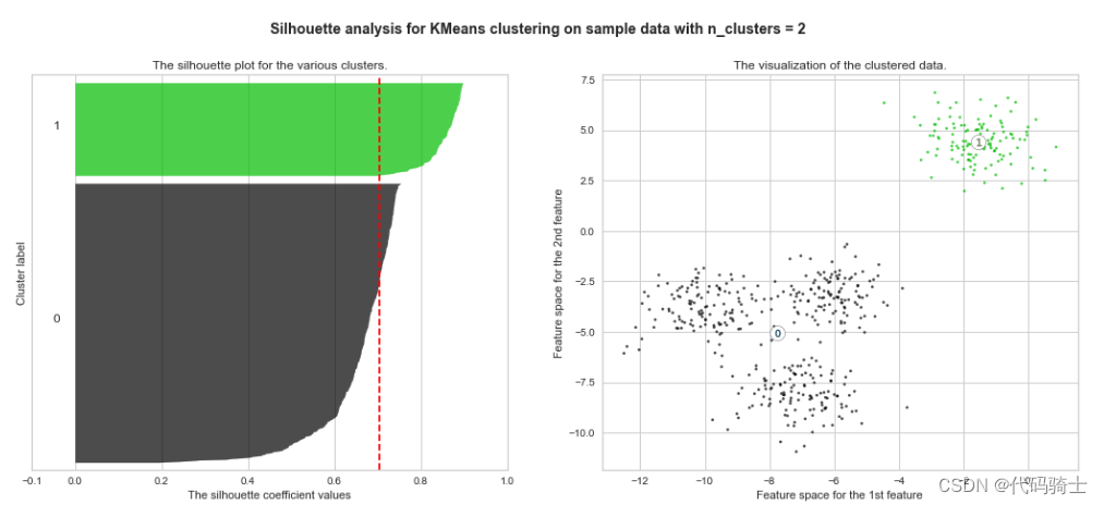
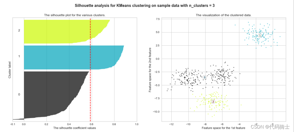
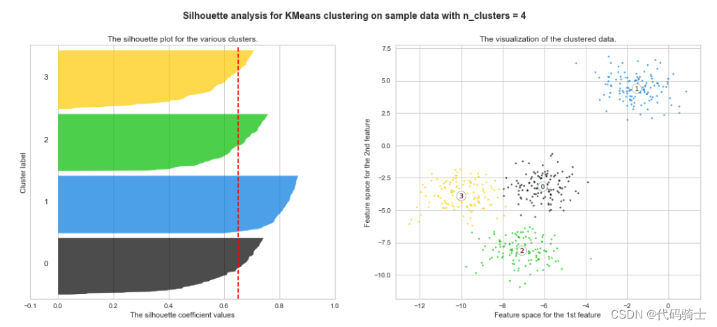
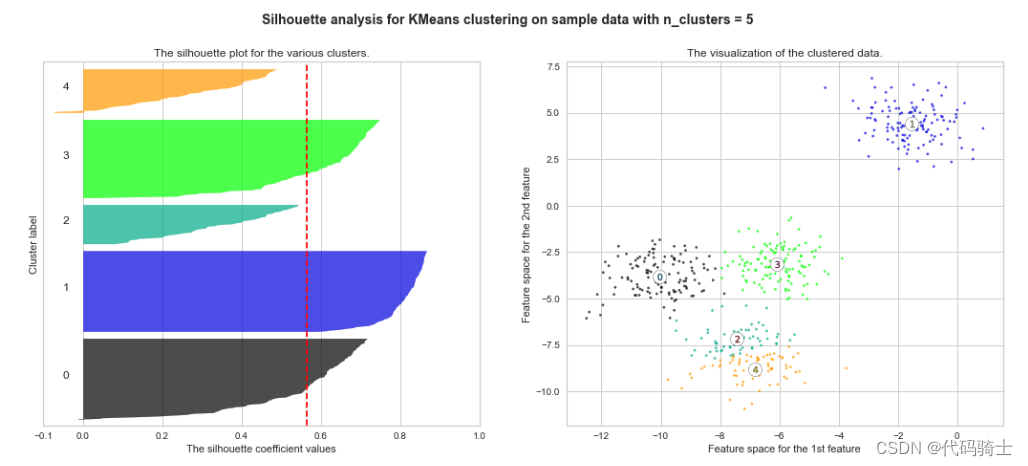
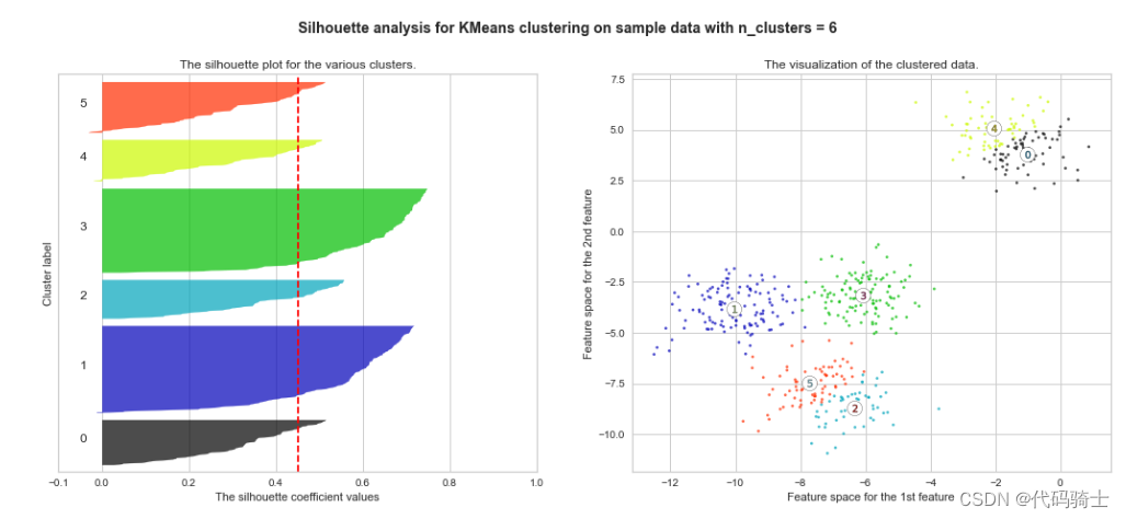
由此可见,既没有出现负值,得分还高的是clusters = 2或clusters = 4。
P32-无监督学习Principal Component AnalysisPCA精简高维数据(降维)
https://www.youtube.com/watch?v=tx34BbqcOuY&list=PLGkfh2EpdoKU3OssXkTl3y7c9tw7jjvHm&index=32
无监督学习中的主成分分析(PCA)是一种常用的降维方法,可以将高维数据精简为低维数据,同时保留原始数据的主要信息。
主成分分析(PCA)是一种无监督技术,用于预处理和降低高维数据集的维度,同时保留原始数据集固有的结构和关系,以便机器学习模型仍然可以从中学习并用于进行准确的预测。
PCA 是一个降维工具,而不是分类器。(PCA是用来对高位数据进行处理的,而不是直接拿来建模的。)在 Scikit-Learn 中,所有分类器和估计器都有一个 predict 方法,而 PCA 没有。你需要在 PCA 转换后的数据上拟合一个分类器。顺便说一下,你可能甚至不需要使用 PCA 来获得良好的分类结果。
PCA 主要应用于强相关的变量。如果变量之间的关系较弱,PCA 无法很好地减少数据量。请参考相关系数矩阵来确定。一般来说,如果大部分相关系数都小于 0.3,PCA 将不会有太大帮助。
from IPython.display import Image
Image(filename='C:\\Users\\86185\\Desktop\\TempDesktop\\研究内容\\Python学习\\Py机深文字教程+源码\\LessonPythonCode-main\\Lesson31-PrincipalComponentAnalysis.jpg')
#C:\\Users\\86185\\Desktop\\TempDesktop\\研究内容\\Python学习\\Py机深文字教程+源码\\LessonPythonCode-main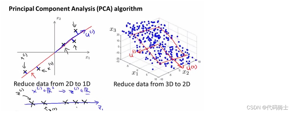
from IPython.display import Image
Image(filename='C:\\Users\\86185\\Desktop\\TempDesktop\\研究内容\\Python学习\\Py机深文字教程+源码\\LessonPythonCode-main\\Lesson31-Principal Component Analysis second principal.gif')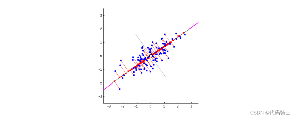
import numpy as np
import matplotlib.pyplot as plt
import seaborn as sns; sns.set(style='white')
%matplotlib inline
%config InlineBackend.figure_format = 'retina'
from sklearn import decomposition
from sklearn import datasets
from mpl_toolkits.mplot3d import Axes3D
# Loading the dataset
iris = datasets.load_iris()
X = iris.data
y = iris.targetfrom IPython.display import Image
Image(filename='C:\\Users\\86185\\Desktop\\TempDesktop\\研究内容\\Python学习\\Py机深文字教程+源码\\LessonPythonCode-main\\Lesson31-iris_with_labels.jpg')
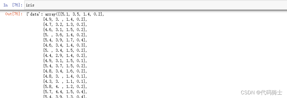
# Let's create a beautiful 3d-plot
fig = plt.figure(1, figsize=(6, 5))
plt.clf()
ax = Axes3D(fig, rect=[0, 0, .95, 1], elev=48, azim=134)
plt.cla()
for name, label in [('Setosa', 0), ('Versicolour', 1), ('Virginica', 2)]:
ax.text3D(X[y == label, 0].mean(),
X[y == label, 1].mean() + 1.5,
X[y == label, 2].mean(), name,
horizontalalignment='center',
bbox=dict(alpha=.5, edgecolor='w', facecolor='w'))
# Change the order of labels, so that they match
y_clr = np.choose(y, [1, 2, 0]).astype(np.float)
ax.scatter(X[:, 0], X[:, 1], X[:, 2], c=y_clr,
cmap=plt.cm.nipy_spectral)
ax.w_xaxis.set_ticklabels([])
ax.w_yaxis.set_ticklabels([])
ax.w_zaxis.set_ticklabels([]);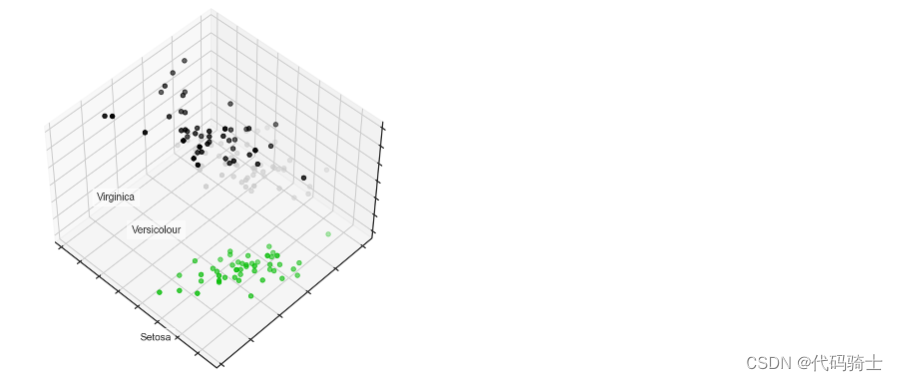
from sklearn.tree import DecisionTreeClassifier
from sklearn.model_selection import train_test_split
from sklearn.metrics import accuracy_score, roc_auc_score
# Train, test splits
X_train, X_test, y_train, y_test = train_test_split(X, y, test_size=.3,
stratify=y,
random_state=42)
# Decision trees with depth = 2
clf = DecisionTreeClassifier(max_depth=2, random_state=42)
clf.fit(X_train, y_train)
preds = clf.predict_proba(X_test)
print('Accuracy: {:.5f}'.format(accuracy_score(y_test,
preds.argmax(axis=1))))Accuracy: 0.88889
数据标准化
from sklearn.preprocessing import MinMaxScaler
scaler = MinMaxScaler()
scaler.fit(X)
data_rescaled = scaler.fit_transform(X)使用PCA
# Using PCA from sklearn PCA
pca = decomposition.PCA(n_components=2)
pca.fit(data_rescaled)
X_pca = pca.transform(data_rescaled)
# Plotting the results of PCA
plt.plot(X_pca[y == 0, 0], X_pca[y == 0, 1], 'bo', label='Setosa')
plt.plot(X_pca[y == 1, 0], X_pca[y == 1, 1], 'go', label='Versicolour')
plt.plot(X_pca[y == 2, 0], X_pca[y == 2, 1], 'ro', label='Virginica')
plt.legend(loc=0);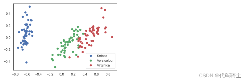
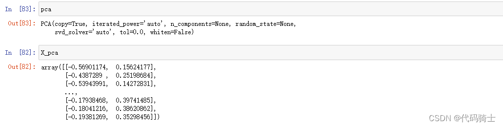
# Test-train split and apply PCA
X_train, X_test, y_train, y_test = train_test_split(X_pca, y, test_size=.3,
stratify=y,
random_state=42)
clf = DecisionTreeClassifier(max_depth=2, random_state=42)
clf.fit(X_train, y_train)
preds = clf.predict_proba(X_test)
print('Accuracy: {:.5f}'.format(accuracy_score(y_test,
preds.argmax(axis=1))))Accuracy: 0.91111
for i, component in enumerate(pca.components_):
print("{} component: {}% of initial variance".format(i + 1,
round(100 * pca.explained_variance_ratio_[i], 2)))
print(" + ".join("%.3f x %s" % (value, name)
for value, name in zip(component,
iris.feature_names)))1 component: 84.14% of initial variance 0.425 x sepal length (cm) + -0.151 x sepal width (cm) + 0.616 x petal length (cm) + 0.646 x petal width (cm) 2 component: 11.75% of initial variance 0.423 x sepal length (cm) + 0.904 x sepal width (cm) + -0.060 x petal length (cm) + -0.010 x petal width (cm)
pca.explained_variance_ratio_array([8.05823175e-01, 1.63051968e-01, 2.13486092e-02, 6.95699061e-03,
1.29995193e-03, 7.27220158e-04, 4.19044539e-04, 2.48538539e-04,
8.53912023e-05, 3.08071548e-05, 6.65623182e-06, 1.56778461e-06,
7.96814208e-08])
plt.figure(figsize=(10,7))
plt.plot(np.cumsum(pca.explained_variance_ratio_), color='k', lw=2)
plt.xlabel('Number of components')
plt.ylabel('Total explained variance')
plt.xlim(0, 4)
#plt.yticks(np.arange(0.8, 1.1, 0.1))
plt.axvline(21, c='b')
plt.axhline(0.95, c='r')
plt.show();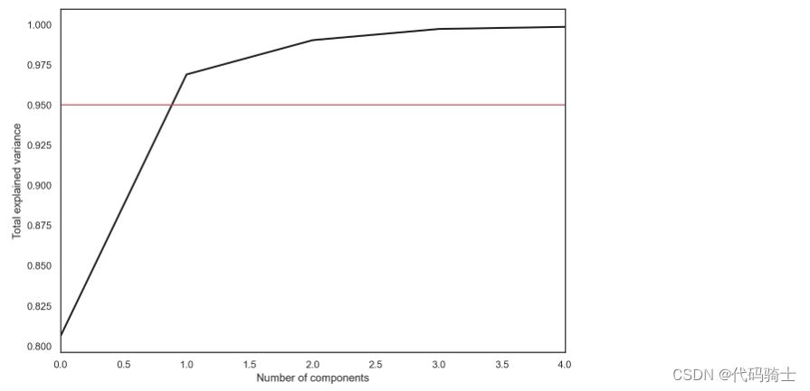
pca.explained_variance_ratio_array([0.84136038, 0.11751808])


 被折叠的 条评论
为什么被折叠?
被折叠的 条评论
为什么被折叠?
 到【灌水乐园】发言


