


前言
在这个项目中,您将构建一个管道,将几幅图像拼接成一个全景图。您还将捕获一组您自己的图像来报告最终的结果。
步骤1 特征检测与描述🍉
本项目的第一步是对序列中的每幅图像分别进行特征检测。回想一下我们在这个类中介绍过的一些特征探测器:哈里斯角、Blob探测器、SIFT探测器等。与检测步骤相结合,就进行了特征描述。您的特性必须对某些转换是不变的。想想你将收集数据集的方式。你需要什么样的不变性?探索在OpenCV中可用的特性描述符实现: SIFT、SURF、ORB等
1.使用cv2.imread读取输入的图像。
2.将图像转换为灰度(例如,使用cv2.cvtColor)以进行特征提取。您也可以通过cv2.resize调整图像的大小(例如,在参考约塞米蒂序列中那样的480像素的高度),以使以下步骤运行得更快。
3.选择您的特征检测器。cv2是一个很好的开始。SIFT_create(或cv2.xfeatures2d。SIFT_Creve在旧的OpenCV版本中)。
4.使用检测和计算方法提取关键点和关键点特征。
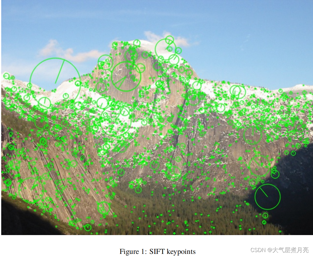
5.图1使用cv2.drawKeypoints可视化了检测到的关键点:
def flt_show(image, title='sift detects'):
    plt.figure(figsize=(10,10)) # Canvas 10x magnification
    plt.title(title,fontsize=20) # title
    plt.axis('off') # Hidden axis
    plt.imshow(cv2.cvtColor(image,cv2.COLOR_BGR2RGB)) # print image
    plt.show() # Display canvas

# 1. Read the input images using cv2.imread.
def feature_detection_and_description(image_path):
    image = cv2.imread(image_path)
    # RGB to Gray
    image = cv2.cvtColor(image,cv2.COLOR_BGR2GRAY)
    # Create detector
    sift_detecter = sift = cv2.SIFT_create()
    # Detection picture
    kp,des = sift.detectAndCompute(image,None) # Keypoints and descriptors
    # Plot key points
    img2 = cv2.drawKeypoints(image,kp,None,(255,0,0),4)
    # show
    flt_show(img2)

    # Release resources
    cv2.waitKey(0)
    cv2.destroyAllWindows()

feature_detection_and_description('yosemite1.jpg')
步骤2 特征匹配和图像对齐🍉
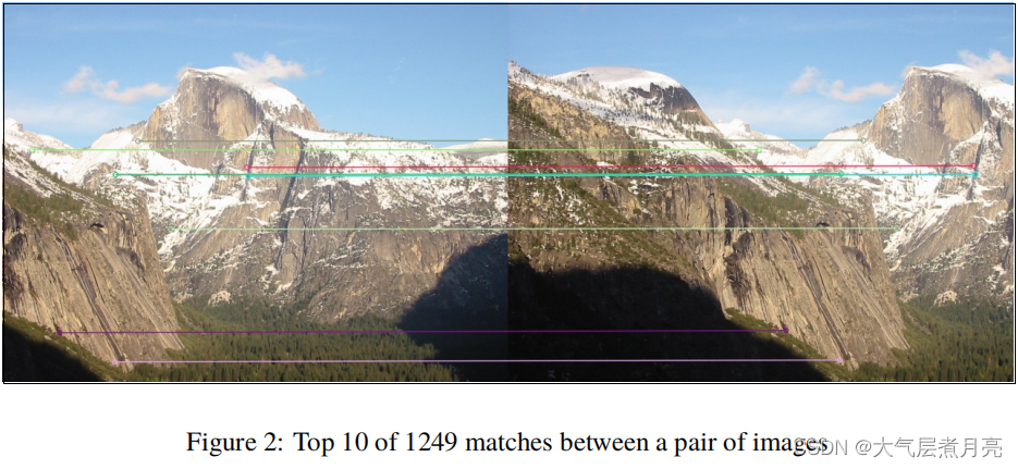
一旦计算出了关键点和特征,代码就需要在连续的图像对之间建立良好的匹配。为此,您需要选择一个距离函数和一个匹配算法。
1.选择一个匹配算法和一个距离函数。强力匹配(cv2。你可以做这个工作,因为你以后会摆脱糟糕的比赛!如果您使用二进制特性,如简短或ORB,看看汉明距离函数(cv2。NORM_HAMMING),否则,只需使用欧几里得距离(cv2。norm_l2 ).
2.使用匹配()方法从一对图像中计算匹配,并提供它们的特征作为输入。选择一对有良好重叠的图像。实际上,按照预定义的顺序(例如从左到右)捕捉图像进行全景拼接是很方便的,这样相邻的图像总是有很好的重叠。
3.使用原始的关键点位置和匹配,以两个m×2数组点1和点2的形式构造对应,这样点1[i]和点2[i]分别在第一和第二幅图像中存储匹配的位置。如果您正在使用建议的OpenCV功能,请查看关键点和DMatch类的接口,以了解如何操作返回对象。
4.现在,从对应关系中估计图像之间的同源性变换。匹配项将会有很多离群值,所以你需要选择一个对离群值很健壮的估计器,比如RANSAC。cv2.findHomography对这一步很有用!
5.最后,用模糊的同源性扭曲其中一幅图像: cv2.warpPerspective。
def detectAndDescribe(image):
    # convert the image to grayscale
    gray = cv2.cvtColor(image, cv2.COLOR_BGR2GRAY)

    # detect and extract features from the image
    descriptor = cv2.SIFT_create()
    (kps, features) = descriptor.detectAndCompute(image, None)

    # convert the keypoints from KeyPoint objects to NumPy
    # arrays
#     kps = np.float32([kp.pt for kp in kps])

    # return a tuple of keypoints and features
    return (kps, features)

def matchKeypoints(kpsA, kpsB, featuresA, featuresB, ratio, reprojThresh):
    # compute the raw matches and initialize the list of actual
    # matches
#     matcher = cv2.DescriptorMatcher_create("BruteForce")
#     rawMatches = matcher.knnMatch(featuresA, featuresB, 2)
#     matches = []
#     # loop over the raw matches
#     for m in rawMatches:
#         # ensure the distance is within a certain ratio of each
#         # other (i.e. Lowe's ratio test)
#         if len(m) == 2 and m[0].distance < m[1].distance * ratio:
#             matches.append((m[0].trainIdx, m[0].queryIdx))

    bf = cv2.BFMatcher(cv2.NORM_L2,crossCheck=True)
    matches = bf.match(featuresA,featuresB)
    goods = sorted(matches,key = lambda x:x.distance)
    # computing a homography requires at least 4 matches
    if len(matches) > 4:
        # construct the two sets of points
#         ptsA = np.float32([kpsA[i] for (_, i) in matches])
#         ptsB = np.float32([kpsB[i] for (i, _) in matches])
        ptsA = np.float32([ kpsA[m.queryIdx].pt for m in goods ]).reshape(-1,1,2)
        ptsB = np.float32([ kpsB[m.trainIdx].pt for m in goods ]).reshape(-1,1,2)
        # compute the homography between the two sets of points
        (H, status) = cv2.findHomography(ptsA, ptsB, cv2.RANSAC,
            reprojThresh)

        # return the matches along with the homograpy matrix
        # and status of each matched point
        return (matches, H, status)

    # otherwise, no homograpy could be computed
    return None

def drawMatches(imageA, imageB, kpsA, kpsB, matches, status):
    img1 = imageA
    img2 = imageB
    if len(matches) > 10:
        src_pts = np.float32([ kpsA[m.queryIdx].pt for m in matches ]).reshape(-1,1,2)
        dst_pts = np.float32([ kpsB[m.trainIdx].pt for m in matches ]).reshape(-1,1,2)

        M, mask = cv2.findHomography(src_pts, dst_pts, cv2.RANSAC,5.0)
        matchesMask = mask.ravel().tolist()

        h,w,_ = img1.shape
        pts = np.float32([ [0,0],[0,h-1],[w-1,h-1],[w-1,0] ]).reshape(-1,1,2)
        draw_params = dict(matchColor = (0,255,0), # draw matches in green color
            singlePointColor = None,
            matchesMask = matchesMask, # draw only inliers
            flags = 2)

        img_matchers = cv2.drawMatches(imageA,kpsA,imageB,kpsB,matches,None,**draw_params)
    # return the visualization
    return img_matchers

def feature_matching_and_image_alignment(imageL, imageR, ratio=0.75, reprojThresh=4.0, showMatches=False):
    imageA, imageB = imageR, imageL
    # local invariant descriptors from them
    (kpsA, featuresA) = detectAndDescribe(imageA)
    (kpsB, featuresB) = detectAndDescribe(imageB)

    # match features between the two images
    M = matchKeypoints(kpsA, kpsB,
        featuresA, featuresB, ratio, reprojThresh)

    # if the match is None, then there aren't enough matched
    # keypoints to create a panorama
    if M is None:
        return None

    # otherwise, apply a perspective warp to stitch the images
    # together
    (matches, H, status) = M
    result = cv2.warpPerspective(imageA, H,
        (imageA.shape[1] + imageB.shape[1], imageA.shape[0]))
    result[0:imageB.shape[0], 0:imageB.shape[1]] = imageB

    # check to see if the keypoint matches should be visualized
    if showMatches:
        vis = drawMatches(imageA, imageB, kpsA, kpsB, matches,
            status)

        # return a tuple of the stitched image and the
        # visualization
        return (result, vis)

    # return the stitched image
    return result

result, vis = feature_matching_and_image_alignment(cv2.imread('yosemite1.jpg'), cv2.imread('yosemite2.jpg'), showMatches=True)
flt_show(vis)
flt_show(result)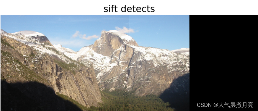
步骤3 图像背景去除🍉
现在您已经将原始图像1和图像2扭曲到图像1的平面上,您需要将它们组合起来以产生无缝的结果。如果你简单地添加图像强度,重叠的区域看起来会很不错,但其他区域看起来会很暗,如图3所示。另一个简单的解决方案是将一幅图像复制粘贴到另一幅图像之上。这还将在边界上创建工件,如图5所示。减少伪影强度的一个解决方案是使用自适应权值来混合图像。靠近每幅图像边界的像素不如位于中心的像素可靠。那么如何将这些像素与与这些像素到相应图像边界的距离成比例的权重进行混合呢?我们提供了get_tinghe_变换函数,它取一个扭曲的RGB图像H×W×3,并产生一个单通道距离函数H×W×1。您可以使用这个函数来计算结果为img1 *权重1+img2*权重2。不要忘记将生成的图像规格化到0…255的范围。尝试使用np.最大值(denom,1.0)以避免除以零。将您的图像转换回无符号的8位整数与img.astype(“uint8”)
def get_distance_transform(img_rgb):
    '''
    Get distance to the closest background pixel for an RGB image
    Input:
        img_rgb : np.array , HxWx3 RGB image
    Output:
        dist : np.array , HxWx1 distance image
            each pixel ’s intensity is proportional to
            its distance to the closest background pixel
            scaled to [0..255] for plotti
    '''
    # Threshold the image : any value above 0 maps into 255
    thresh = cv2.threshold(img_rgb , 0 , 255 , cv2 . THRESH_BINARY )[1]
    # Collapse the color dimension
    thresh = thresh.any(axis =2)
    # Pad to make sure the border is treated as background
    thresh = np.pad(thresh, 1, mode='maximum')
    # Get distance transform
    dist = distance_transform_edt(thresh) [1: -1 , 1: -1]
    # HxW -> HxWx1
    dist = dist[: , : , None ]
    return dist / dist . max () * 255.0

def getMaskResult(result, show=False):
    mask = get_distance_transform(result)

    locs = np.where(mask>0)
    xmin = np.min(locs[1])
    xmax = np.max(locs[1])
    ymin = np.min(locs[0])
    ymax = np.max(locs[0])
    result_mask = result[ymin:ymax, xmin:xmax]
    if show:
        flt_show(result, 'before')
        flt_show(result_mask, 'after')
    return result_mask
result_mask = getMaskResult(result, True)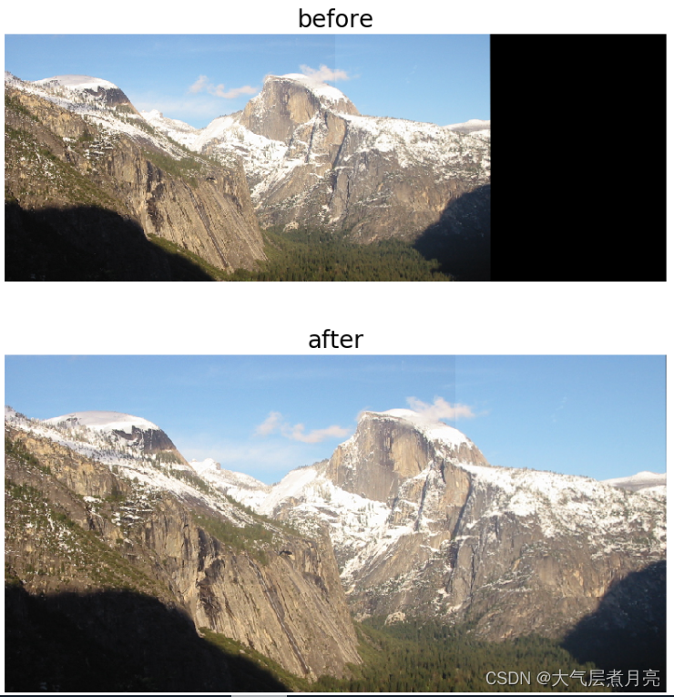
步骤4 缝合多张图像🍉
拼接n个图像的一个简单方法是从左到右对序列进行排序,并逐步应用成对拼接:如果拼接每一对相邻图像,将得到n个−1的全景图。您可以一次又一次地对这些图像应用相同的拼接过程,直到您只留下一个宽的全景图。您只需要在它上面添加一个for循环。
imageList = [cv2.imread('yosemite1.jpg'), cv2.imread('yosemite2.jpg'), cv2.imread('yosemite3.jpg'),cv2.imread('yosemite4.jpg')]

temp_image = feature_matching_and_image_alignment(imageList[0], imageList[1])
temp_image = getMaskResult(temp_image)
flt_show(temp_image1, title='Step 1')
for i in range(2, 4):
    temp_image = feature_matching_and_image_alignment(temp_image, imageList[i])
    temp_image = getMaskResult(temp_image)
    flt_show(temp_image, title='Step {}'.format(i))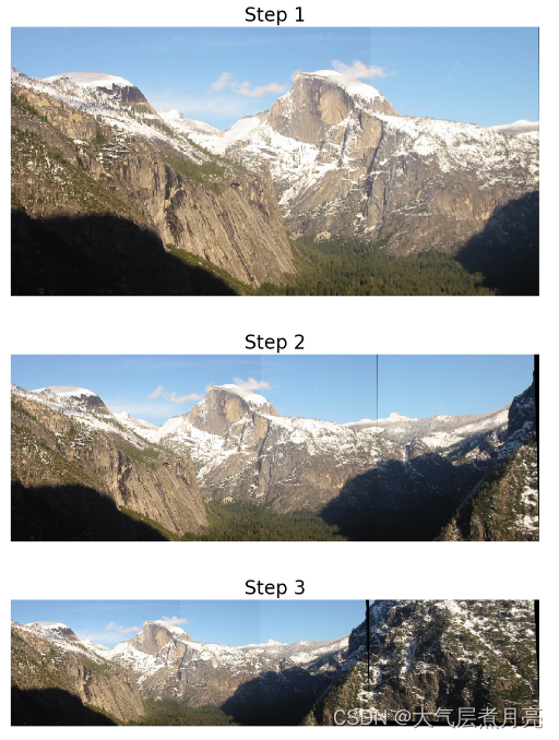
步骤5 创建您自己的全景图,并讨论设置和结果。🍉
请注意,这一步将主要根据您提供的讨论进行分级(例如,只捕获一些图像并在不编写的情况下生成结果不会给您很多分数)。为了获得一个好的全景,在捕捉自己的图像时有几件事需要考虑。
imageList = [cv2.imread('1.png'), cv2.imread('2.png'), cv2.imread('3.png'),cv2.imread('4.png'), cv2.imread('5.png')]
temp_image = feature_matching_and_image_alignment(imageList[0], imageList[1])
temp_image = getMaskResult(temp_image)
flt_show(temp_image, title='Step 1')
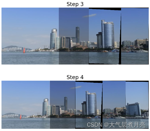
for i in range(2, 5):
temp_image = feature_matching_and_image_alignment(temp_image, imageList[i])
temp_image = getMaskResult(temp_image)
flt_show(temp_image, title='Step {}'.format(i))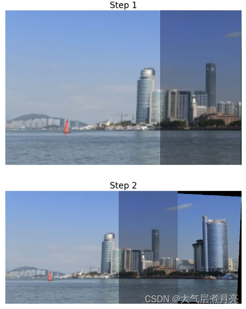
# # # #发表评论
- 1。这已经在步骤4中完成了。
- 2。数据集捕捉了沿河的建筑风景,具有良好的视野和易于区分的特征。
- 3。相邻的图片有很好的重叠。
- 4. 摄像机角度的变化容易引起同态现象。如果天气晴朗,最好待在室外,视野开阔,位置好,光线也明亮。只要两幅图像之间的特征明显,摄像机是否自由移动并不重要。
当三张以上的图片拼接在一起时,由于黑色背景的原因,图像与其他图像的拼接会有很多困难。背景剔除可以解决这个问题。
感谢观看!由于是作业的缘故,文中可能有极少部分会出现语义不通顺的情况,但对本文的目的没有什么影响。


 1万+
1万+


 被折叠的 条评论
为什么被折叠?
被折叠的 条评论
为什么被折叠?
 到【灌水乐园】发言


