《斯坦福数据挖掘教程·第三版》读书笔记（英文版）Chapter 12 Large-Scale Machine Learning

来源：《斯坦福数据挖掘教程·第三版》对应的公开英文书和PPT

Chapter 12 Large-Scale Machine Learning

Algorithms called “machine learning” not only summarize our data; they are perceived as learning a model or classifier from the data, and thus discover something about data that will be seen in the future.

The term unsupervised refers to the fact that the input data does not tell the clustering algorithm what the clusters should be. In supervised machine learning, the available data includes information about the correct way to classify at least some of the data. The data classified already is called the training set.

The data to which a machine-learning algorithm is applied is called a training set. A training set consists of a set of pairs $(x,y)$, called training examples, where

• x is a vector of values, often called a feature vector, or simply an input. Each value, or feature, can be categorical (values are taken from a set of discrete values, such as {red, blue, green}) or numerical (values are integers or real numbers).
• y is the class label, or simply output, the classification value for x.

The objective of the ML process is to discover a function $y=f(x)$ that best predicts the value of y associated with each value of x. The type of y is in principle arbitrary, but there are several common and important cases.

1. y is a real number. In this case, the ML problem is called regression.
2. y is a Boolean value: true-or-false, more commonly written as +1 and −1, respectively. In this class the problem is binary classification.
3. y is a member of some finite set. The members of this set can be thought of as “classes,” and each member represents one class. The problem is multiclass classification.
4. y is a member of some potentially infinite set, for example, a parse tree for x, which is interpreted as a sentence.

There are many forms of ML algorithms, and we shall not cover them all here. Here are the major classes of such algorithms, each of which is distinguished by the form by which the function $f$ is represented.

1. Decision trees. The form of $f$ is a tree, and each node of the tree has a function of x that determines to which child or children the search must proceed. Decision trees are suitable for binary and multiclass classification, especially when the dimension of the feature vector is not too large (large numbers of features can lead to overfitting).

2. Perceptrons are threshold functions applied to the components of the vector $x=[x_1,x_2,...,x_n]$. A weight $w_i$is associated with the ith component, for each $i=1,2,...,n$, and there is a threshold $\theta$. The output is +1 if

   $$\sum _{i=1}^n{w}_i{x}_i>\theta$$

   and the output is −1 if that sum is less than $\theta$. A perceptron is suitable for binary classification, even when the number of features is very large.

3. Neural nets are acyclic networks of perceptrons, with the outputs of some perceptrons used as inputs to others. These are suitable for binary or multiclass classification, since there can be several perceptrons used as output, with one or more indicating each class.

4. Instance-based learning uses the entire training set to represent the function $f$. The calculation of the label y associated with a new feature vector x can involve examination of the entire training set, although usually some preprocessing of the training set enables the computation of $f(x)$ to proceed efficiently. We shall consider an important kind of instance-based learning, k-nearest-neighbor.

5. Support-vector machines are an advance over the algorithms traditionally used to select the weights and threshold. The result is a classifier that tends to be more accurate on unseen data.

The validation set is used to help design the model, while the test set is used only to determine how good the model is. The problem addressed by a validation set is that many machine-learning algorithms tend to overfit the data; they pick up on artifacts that occur in the training set but that are atypical of the larger population of possible data. By using the validation set, and seeing how well the classifier works on that, we can tell if the classifier is overfitting the data. If so, we can restrict the machine-learning algorithm in some way. For instance, if we are constructing a decision tree, we can limit the number of levels of the tree.

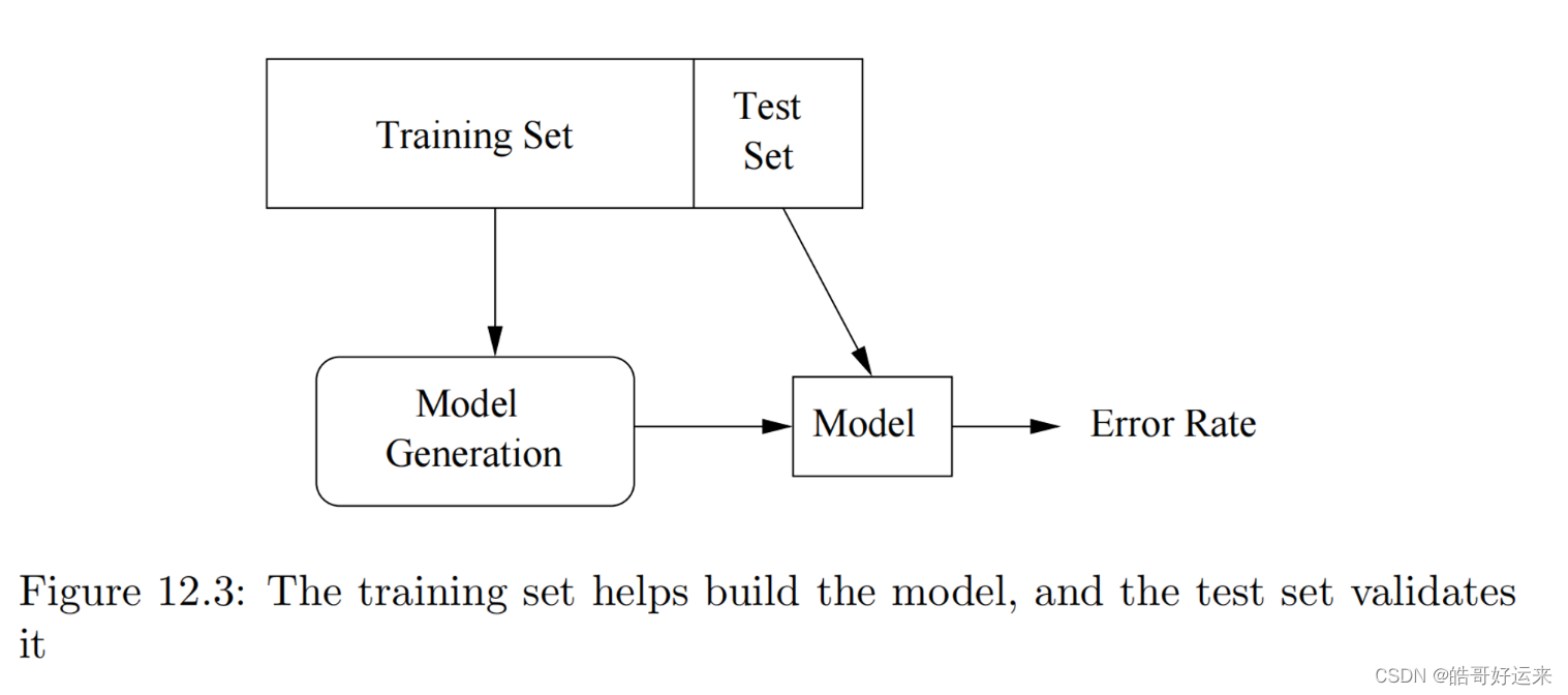
We can repeat the train-then-test process several times using the same data, if we divide the data into $k$ equal-sized chunks. In turn, we let each chunk be the test data, and use the remaining $k-1$ chunks as the training data. This training architecture is called cross-validation.

We use a batch learning architecture. That is, the entire training set is available at the beginning of the process, and it is all used in whatever way the algorithm requires to produce a model once and for all. The alternative is on-line learning, where the training set arrives in a stream and, like any stream, cannot be revisited after it is processed. In on-line learning, we maintain a model at all times. As new training examples arrive, we may choose to modify the model to account for the new examples. On-line learning has the advantages that it can

1. Deal with very large training sets, because it does not access more than one training example at a time.
2. Adapt to changes in the population of training examples as time goes on. For instance, Google trains its spam-email classifier this way, adapting the classifier for spam as new kinds of spam email are sent by spammers and indicated to be spam by the recipients.

An enhancement of on-line learning, suitable in some cases, is active learning. Here, the classifier may receive some training examples, but it primarily receives unclassified data, which it must classify. If the classifier is unsure of the classification (e.g., the newly arrived example is very close to the boundary), then the classifier can ask for ground truth at some significant cost. For instance, it could send the example to Mechanical Turk and gather opinions of real people. In this way, examples near the boundary become training examples and can be used to modify the classifier.

Perceptrons

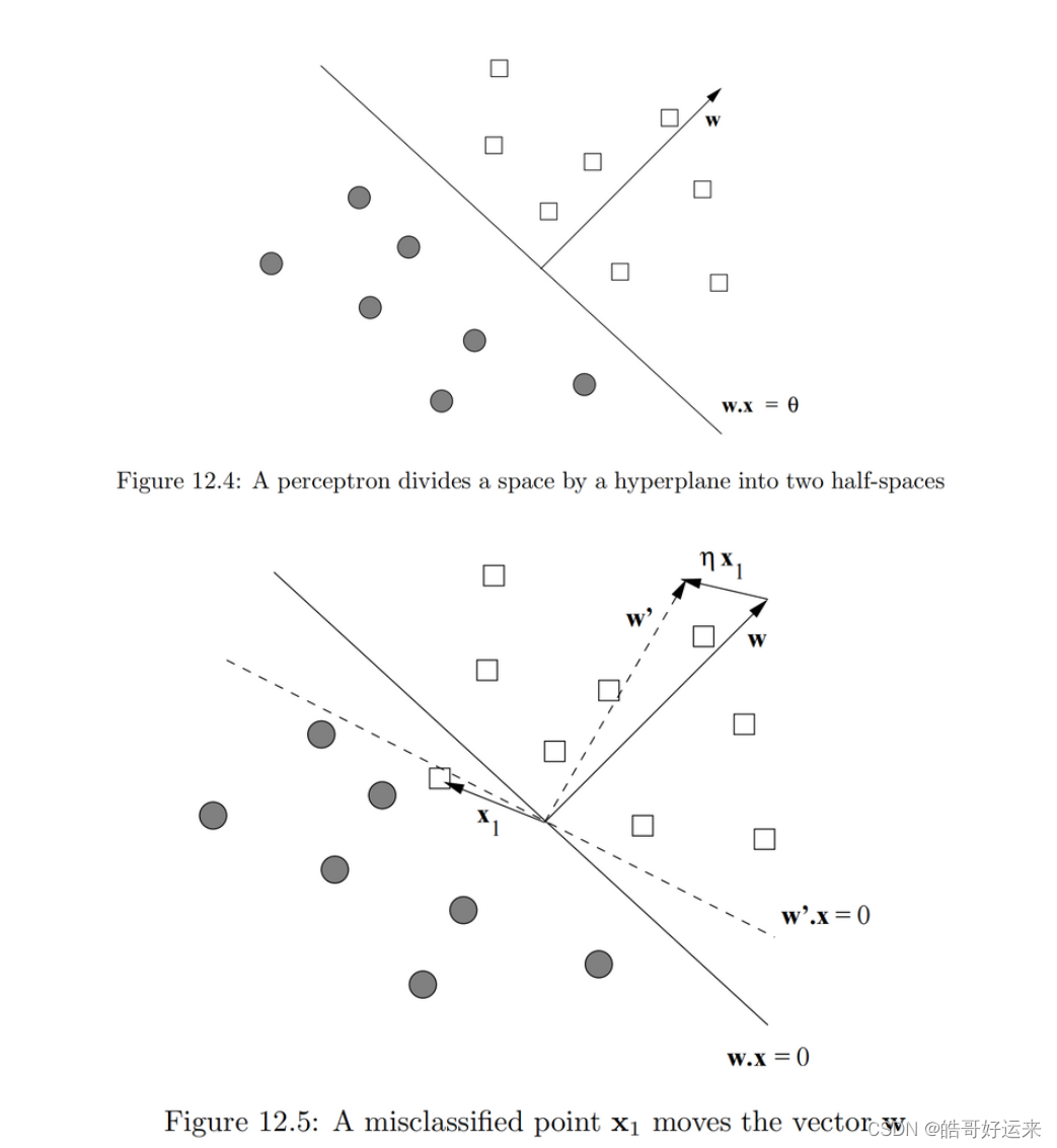
A perceptron is a linear binary classifier. Its input is a vector $x=[x1,x2,...,xd]$ with real-valued components. Associated with the perceptron is a vector of weights $w=[w1,w2,...,wd]$, also with real-valued components. Each perceptron has a threshold $\theta$.

The weight vector w defines a hyperplane of dimension $d-1$ – the set of all points x such that $w\cdot x=\theta ,$ as suggested in Fig. 12.4. Points on the positive side of the hyperplane are classified +1 and those on the negative side are classified −1. A perceptron classifier works only for data that is linearly separable, in the sense that there is some hyperplane that separates all the positive points from all the negative points. If there are many such hyperplanes, the perceptron will converge to one of them, and thus will correctly classify all the training points. If no such hyperplane exists, then the perceptron cannot converge to any hyperplane. In the next section, we discuss support-vector machines, which do not have this limitation; they will converge to some separator that, although not a perfect classifier, will do as well as possible under the
metric to be described in SVM.

Here are some common tests for termination.

1. Terminate after a fixed number of rounds.
2. Terminate when the number of misclassified training points stops changing.
3. Withhold a test set from the training data, and after each round, run the perceptron on the test data. Terminate the algorithm when the number of errors on the test set stops changing.

Another technique that will aid convergence is to lower the training rate as the number of rounds increases. For example, we could allow the training rate $\eta$ to start at some initial ${\eta }_0$ and lower it to ${\eta }_0/(1+c_t)$ after the t-th round, where $c$ is some small constant.

There are many other rules one could use to adjust weights for a perceptron. Not all possible algorithms are guaranteed to converge, even if there is a hyperplane separating positive and negative examples. One that does converge is called Winnow, and that rule will be described here. Winnow assumes that the feature vectors consist of 0’s and 1’s, and the labels are +1 or −1. Unlike the basic perceptron algorithm, which can produce positive or negative components in the weight vector w, Winnow produces only positive weights.

We shall give the details of the algorithm using the factors 2 and 1/2, for the cases where we want to raise weights and lower weights, respectively. Start the Winnow Algorithm with a weight vector $w=[w1,w2,...,wd]$ all of whose components are 1, and let the threshold $\theta$equal $d$, the number of dimensions of the vectors in the training examples. Let $(x,y)$ be the next training example to be considered, where $x=[x1,x2,...,xd]$.

1. If $w\cdot x>\theta$ and y = +1, or $w\cdot x<\theta$ and y = −1, then the example is correctly classified, so no change to w is made.
2. If $w\cdot x\le \theta$, but y = +1, then the weights for the components where x has 1 are too low as a group. Double each of the corresponding components of w. That is, if $x_i=1$ then set $w_i=2w_i$.
3. If $w\cdot x\ge \theta$, but y = −1, then the weights for the components where x has 1 are too high as a group. Halve each of the corresponding components of w. That is, if $x_i=1$ then set $w_i=w_i/2$.

An example is shown in Fig. 12.11. In this example, points of the two classes mix near the boundary so that any line through the points will have points of both classes on at least one
of the sides.

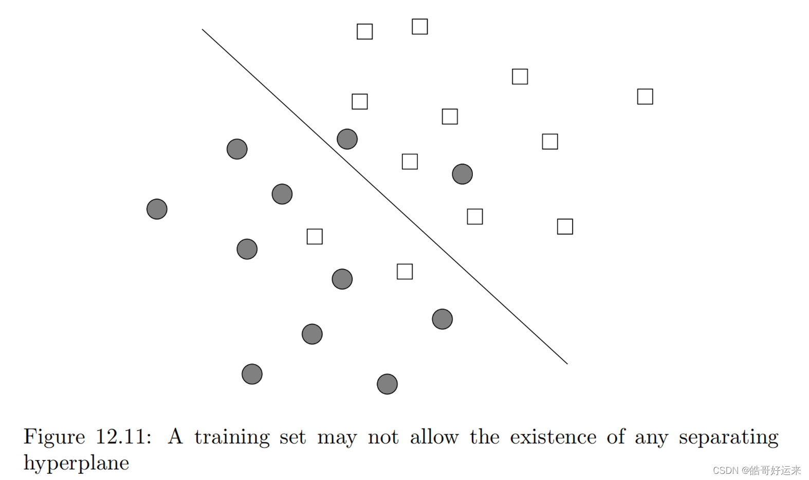
In principle, possible to find some function on the points that transforms them to another space where they are linearly separable. However, doing so could well lead to overfitting, the situation where the classifier works very well on the training set, because it has been carefully designed to handle each training example correctly. However, because the classifier is exploiting details of the training set that do not apply to other examples that must be classified in the future, the classifier will not perform well on new data.

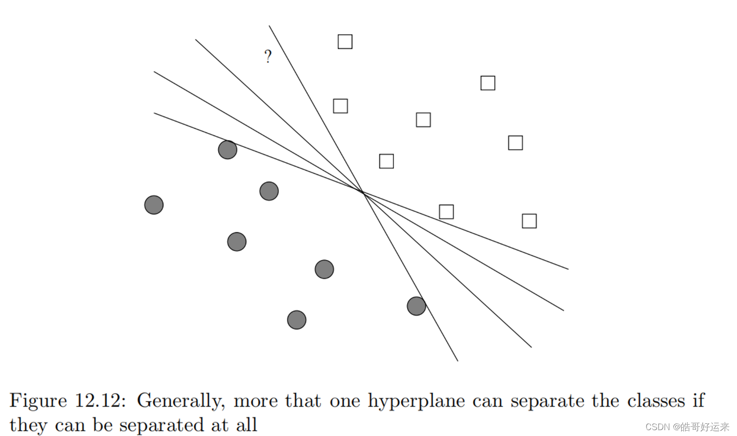
Usually, if classes can be separated by one hyperplane, then there are many different hyperplanes that will separate the points. However, not all hyperplanes are equally good. For instance, if we choose the hyperplane that is furthest clockwise, then the point indicated by “?” will be classified as a circle, even though we intuitively see it as closer to the squares.

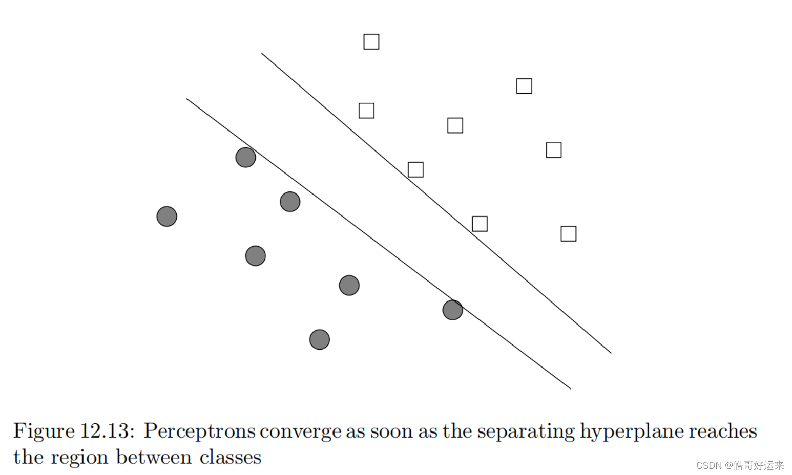
Yet another problem is illustrated by Fig. 12.13. Most rules for training a perceptron stop as soon as there are no misclassified points. As a result, the chosen hyperplane will be one that just manages to classify some of the points correctly. For instance, the upper line in Fig. 12.13 has just managed to accommodate two of the squares, and the lower line has just managed to accommodate two of the circles. If either of these lines represent the final weight vector, then the weights are biased toward one of the classes. That is, they correctly classify the points in the training set, but the upper line would classify new squares that are just below it as circles, while the lower line would classify circles just above it as squares.

SUPPORT-VECTOR MACHINES

We can view a support-vector machine, or SVM, as an improvement on the perceptron that is designed to address the problems mentioned in Section 12.2.7. An SVM selects one particular hyperplane that not only separates the points in the two classes, but does so in a way that maximizes the margin – the distance between the hyperplane and the closest points of the training set.

The goal of an SVM is to select a hyperplane $w\cdot x+b=0$ that maximizes the distance γ between the hyperplane and any point of the training set.1 The idea is suggested by Fig. 12.14. There, we see the points of two classes and a hyperplane dividing them.

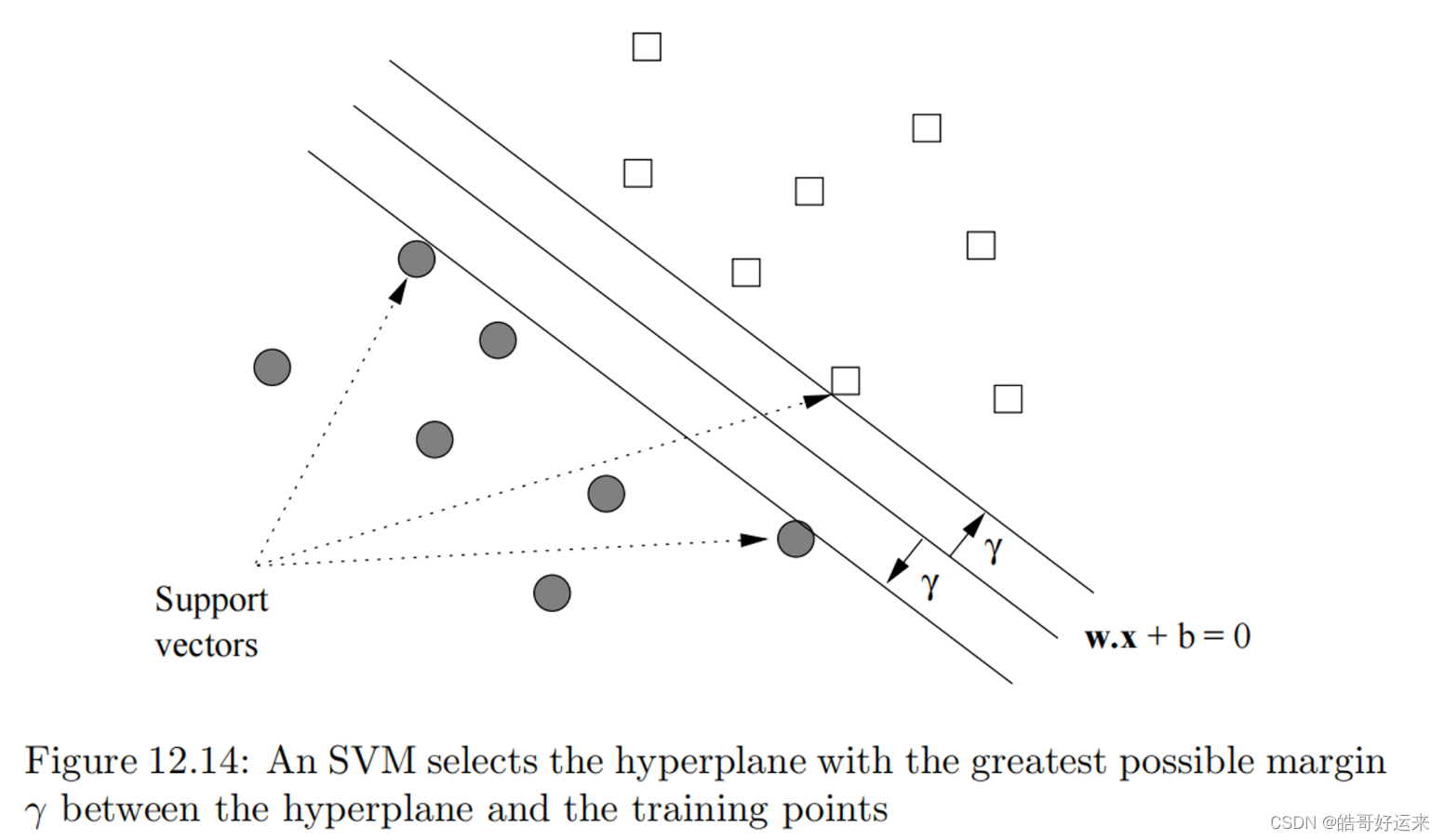
Intuitively, we are more certain of the class of points that are far from the separating hyperplane than we are of points near to that hyperplane. Thus, it is desirable that all the training points be as far from the hyperplane as possible (but on the correct side of that hyperplane, of course). An added advantage of choosing the separating hyperplane to have as large a margin as possible is that there may be points closer to the hyperplane in the full data set but not in the training set. If so, we have a better chance that these points will be classified properly than if we chose a hyperplane that separated the training points but allowed some points to be very close to the hyperplane itself. In that case, there is a fair chance that a new point that was near a training point that was also near the hyperplane would be misclassified.

A tentative statement of our goal is:

Given a training set $(x_1,y_1),(x_2,y_2),...,(x_n,y_n)$, maximize γ (by varying w and b) subject to the constraint that for all $i=1,2,...,n$,

$$y_i(w\cdot x_i+b)\ge \gamma$$

Notice that $y_i$, which must be +1 or −1, determines which side of the hyperplane the point $x_i$ must be on, so the ≥ relationship to γ is always correct. However, it may be easier to express this condition as two cases: if y = +1, then $w\cdot x+b\ge \gamma$, and if y = −1, then $w\cdot x+b\le -\gamma$.
Unfortunately, this formulation doesn’t really work properly. The problem is that by increasing w and b, we can always allow a larger value of γ. For example, suppose that w and b satisfy the constraint above. If we replace w by 2w and b by 2b, we observe that for all $i,y_i$， $((2w)\cdot x_i+2b))\ge 2\gamma$. Thus, 2w and 2b is always a better choice than w and b, so there is no best choice and no maximum γ.

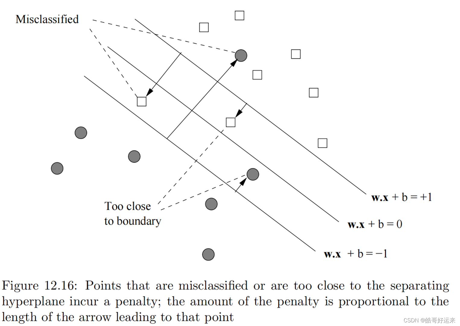
The solution to the problem that we described intuitively above is to normalize the weight vector w. That is, the unit of measure perpendicular to the separating hyperplane is the unit vector $w/||w||$ . Recall that $||w||$ is the Frobenius norm, or the square root of the sum of the squares of the components of w. We shall require that w be such that the parallel hyperplanes that just touch the support vectors are described by the equations $w\cdot x+b=+1$ and $w\cdot x+b=-1$，as suggested by Fig. 12.15. We shall refer to the hyperplanes defined by these two equations as the upper and lower hyperplanes, respectively.

It looks like we have set $\gamma =1$. But since we are using w as the unit vector, the margin γ is the number of “units,” that is, steps in the direction w needed to go between the separating hyperplane and the parallel hyperplanes. Our goal becomes to maximize γ, which is now the multiple of the unit vector $w/||w||$ between the separating hyperplane and the upper and lower hyperplanes. Our first step is to demonstrate that maximizing γ is the same as minimizing
$w/||w||$ .

Consider one of the support vectors, say $x_2$ shown in Fig. 12.15. Let $x_1$ be the projection of $x_2$ onto the upper hyperplane, also as suggested by Fig. 12.15. Note that $x_1$ need not be a support vector or even a point of the training set. The distance from $x_2$ to $x_1$ in units $w/||w||$of is 2γ. That is,

$$x_1=x_2+2\gamma \frac{w}{||w||}$$

Since $x_1$ is on the hyperplane defined by $w\cdot x+b=+1$, we know that. If we substitute for $x_1$ using Equation 12.1, we get

$$w\cdot (x_2+2\gamma \frac{w}{||w||})+b=1$$

Regrouping terms, we see,

$$w\cdot x_2+b+2\gamma \frac{w\cdot w}{||w||}=1$$

we know that $x_2$ is on the lower hyperplane, $w\cdot x+b=-1$. If we move this −1 from left
to right in Equation 12.2 and then divide through by 2, we conclude that

$$\gamma \frac{w\cdot w}{||w||}=1$$

$$\gamma =\frac{1}{||w||}$$

Given a training set $(x_1,y_1),(x_2,y_2),...,(x_n,y_n)$, minimize $||w||$ (by varying w and b) subject to the constraint that for all $i=1,2,...,n$,

$$y_i(w\cdot x_i+b)\ge 1$$

We also see two points that, while they are classified correctly, are too close to the separating hyperplane. We shall call all these points bad points.

Each bad point incurs a penalty when we evaluate a possible hyperplane. The amount of the penalty, in units to be determined as part of the optimization process, is shown by the arrow leading to the bad point from the hyperplane on the wrong side of which the bad point lies. That is, the arrows measure the distance from the hyperplane $w\cdot x+b=1$ or $w\cdot x+b=-1$. The former is the baseline for training examples that are supposed to be above the separating hyperplane (because the label y is +1), and the latter is the baseline for points that are supposed to be below (because y = −1).

Thus, we shall consider how to minimize the particular function，

f ( w , b ) = 1 2 ∑ j = 1 d w i 2 + C ∑ i = 1 n { 0 , 1 − y i ( ∑ j = 1 n w j x i j + b ) } f(w,b)=\frac{1}{2}\sum_{j=1}^{d}w_i^2+C\sum_{i=1}^{n}\{0,1-y_i(\sum_{j=1}^{n}w_jx_{ij}+b)\} f(w,b)=21​j=1∑d​wi2​+Ci=1∑n​{0,1−yi​(j=1∑n​wj​xij​+b)}

The first term encourages small w , while the second term, involving the constant C that must be chosen properly, represents the penalty for bad points in a manner to be explained below. We assume there are n training examples $(x_i,y_i)$ for $i=1,2,...,n$, and $x_i=[x_{i1},x_{i2},...,x_{id}]$. Also, as before, $w=[w_1,w_2,...,w_d]$. Note that the two summations ${\sum }_{j=1}^d$ express the dot product of vectors.
The constant C, called the regularization parameter, reflects how important misclassification is. Pick a large C if you really do not want to misclassify points, but you would accept a narrow margin. Pick a small C if you are OK with some misclassified points, but want most of the points to be far away from the boundary (i.e., the margin is large).

We must explain the penalty function (second term) in Equation 12.4. The summation over i has one term for each training example $x_i$.

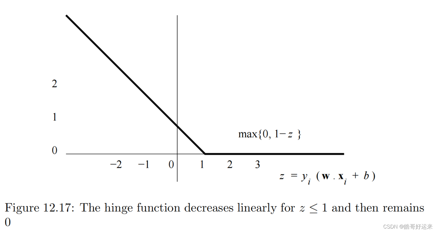
L ( x i , y i ) = m a x { 0 , 1 − y i ( ∑ j = 1 d w j x i j + b ) } L(x_i, y_i) = max\{0, 1 − y_i(\sum_{j=1}^dw_jx_{ij}+b)\} L(xi​,yi​)=max{0,1−yi​(j=1∑d​wj​xij​+b)}

$L$ is the hinge function, suggested in Fig. 12.17, and we call its value the hinge loss. Let $z_i=y_i({\sum }_{j=1}^d{w}_j{x}_{ij}+b)$. When $z_i$ is 1 or more, the value of $L$ is 0. But for smaller values of $z_i$
, L rises linearly as $z_i$ decreases.

Since we shall have need to take the derivative with respect to each $w_j$ of$L(x_i,y_i)$, note that the derivative of the hinge function is discontinuous. It is $-y_i{x}_{ij}$ for $z_i<1$ and 0 for $z_i>1$. That is,

$$\frac{\partial L}{\partial w_j}=if{y}_i(\sum _{j=1}^d{w}_j{x}_{ij}+b)\ge 1then0else-y_i{x}_{ij}$$

SVM Solutions by Gradient Descent

The derivative $\frac{\partial f}{\partial w_j}$ of the first term in Equation 12.4, ${\sum }_{j=1}^d{w}_i^2$, is easy, it is $w_j$ . However, the second term involves the hinge function, so it is harder to express. We shall use an if-then expression to describe these derivatives, as in Equation 12.5. That is:

$$\frac{\partial f}{\partial w_j}=w_i+C\sum _{i=1}^n(if{y}_i(\sum _{j=1}^d{w}_j{x}_{ij}+b)\ge 1then0else-y_i{x}_{ij})$$

Note that this formula gives us a partial derivative with respect to each component of w, including $w_{d+1},$ which is b, as well as to the weights $w_1,w_2,...,w_d$. We continue to use b instead of the equivalent $w_{d+1}$ in the if-then condition to remind us of the form in which the desired hyperplane is described.
To execute the gradient-descent algorithm on a training set, we pick:

1. Values for the parameters C and η.
2. Initial values for w, including the (d + 1)st component b.

Then, we repeatedly:

(a) Compute the partial derivatives of $f(w,b)$ with respect to the $w_j$ ’s.
(b) Adjust the values of w by subtracting $\eta \frac{\partial f}{\partial w_j}$ from each $w_j$ .

Learning from Nearest Neighbors

Normally, we provide a function (the kernel function) of the distance between the query example and its nearest neighbors in the training set, and use this function to weight the
neighbors.

Suppose we use a method with k nearest neighbors, and x is the query point.
Let $x_1,x_2,...,x_k$ be the k nearest neighbors of x, and let the weight associated
with training point $(x_i,y_i)$ be $w_i$. Then the estimate of the label y for x is
${\sum }_{i=1}^k{w}_i{y}_i/{\sum }_{i=1}^k{w}_i$. Note that this expression gives the weighted average of the labels of the k nearest neighbors.

Weighted Average of the Two Nearest Neighbors. We again choose two nearest neighbors, but we weight them in inverse proportion to their distance from the query point. Suppose the two neighbors nearest to query point x are $x_1$ and $x_2$. Suppose first that $x_1<x<x_2$. Then the weight of $x_1$, the inverse of its distance from x, is $1/(x-x_1)$, and the weight of $x_2$ is $1/(x_2-x)$. The weighted average of the labels is

$$(\frac{y_1}{x-x_1}+\frac{y_1}{x_2-x})/(\frac{1}{x-x_1}+\frac{1}{x_2-x})$$

When both nearest neighbors are on the same side of the query $x$, the same weights make sense, and the resulting estimate is an extrapolation. In general, when points are unevenly spaced, we can find query points in the interior where both neighbors are on one side.

A way to construct a continuous function that represents the data of a training set well is to consider all points in the training set, but weight the points using a kernel function that decays with distance. A popular choice is to use a normal distribution (or “bell curve”), so the weight of a training point x when the query is q is $e^{{-(x-q)}^2/{\sigma }^2}$. Here $\sigma$ is the standard deviation of the distribution (a parameter you select) and the query q is the mean. Roughly, points within distance σ of q are heavily weighted, and those further away have little weight. There is an advantage to using a kernel function, such as the normal distribution, that is continuous and defined for all points in the training set; doing so assures that the resulting function learned from the data is itself continuous.

Unfortunately, for high-dimensional data, there is little that can be done to avoid searching a large portion of the data. Two ways to deal with the “curse” are the following:

1. VA Files. Since we must look at a large fraction of the data anyway in order to find the nearest neighbors of a query point, we could avoid a complex data structure altogether. Accept that we must scan the entire file, but do so in a two-stage manner. First, a summary of the file is created, using only a small number of bits that approximate the values of each component of each training vector. For example, if we use only the high-order (1/4)th of the bits in numerical components, then we can create a file that is (1/4)th the size of the full dataset. However, by scanning this file we can construct a list of candidates that might be among the k nearest neighbors of the query q, and this list may be a small fraction of the entire dataset. We then look up only these candidates in the complete file, in order to determine which k are nearest to q.
2. Dimensionality Reduction. We may treat the vectors of the training set as a matrix, where the rows are the vectors of the training example, and the columns correspond to the components of these vectors. Apply one of the dimensionality-reduction techniques of Chapter 11, to compress the vectors to a small number of dimensions, small enough that the techniques for multidimensional indexing can be used. Of course, when processing a query vector $q$, the same transformation must be applied to q before searching for $q$’s nearest neighbors.

Decision Trees

We can formalize the property we would like for a node by the notion of impurity. There are many impurity measures we could use, but they all have the property that they are 0 for a node that is reached only by training examples with a single class. Here are three of the most common impurity measures. Each applies to a node reached by training examples with n classes, with $p_i$ being the fraction of those training examples that belong the i-th class, for $i=1,2,...,n$.

1. Accuracy: the fraction of the reaching inputs that are correctly classified, or $1-max(p_1,p_2,...,p_n)$.
2. GINI Impurity: $1-{\sum }_{n=1}^n(p_i{)}^2$.
3. Entropy: ${\sum }_{i=1}^n{p}_{i}lo{g}_2(1/p_i)$.

Suppose we are given a node of the decision tree that is reached by a subset of the training examples. If the node is pure, i.e., all these training examples have the same output, then we make the node a leaf with that output as value. However, if the impurity is greater than zero, we want to find the test that gives the greatest reduction in impurity. When selecting this test, we are free to choose any feature of the input vector. If we choose a numerical feature, we can choose any constant to divide the training examples into two sets, one going to the left child and the other going to the right child. Alternatively, if we choose a categorical feature, then we may choose any set of values for the membership test.

To select the best breakpoint, we

1. Order the training examples according to their value of A. Let the values of A in this order be .$a_1,a_2,...,a_n$
2. For $j=1,2,...,n$, compute the number of training examples in each class among $a_1,a_2,...,a_j$ . Note that these counts can be done incrementally, since the count for a class after the jth example is either the same as the count for $j-1$ (if the jth example in not in this class) or one more than the count for $j-1$ (if the jth example is in this class).
3. From the counts computed in the previous step, compute the weighted average impurity assuming the test sends the first j training examples to the left child and the remaining $n-j$ examples to the right node.
4. Select that value of j that minimizes the weighted-average impurity. However, note that not every possible value of j can be used at this step, since it is possible that $a_j=a_j+1$. We need to restrict our choice of j to those values such that $a_j<a_j+1$, so that we can use $A<(a_j+a_j+1)/2$ as the comparison.

If we design a decision tree using as many levels as needed so that each leaf is pure, we are likely to have overfit to the training data. If we can verify our design using other examples – either a test set that we have withheld from the training data or a set of new data – we have the opportunity to simplify the tree and at the same time limit the overfitting.

Find a node N that has only leaves as children. Build a new tree by replacing N and its children by a leaf, and give that leaf its majority class as its output. Then, compare the performance of the old and new trees on data that was not used as training examples when we designed the tree. If there is little difference between the error rates of the old and new trees, then the decision made at the node N probably contributed to overfitting and was not addressing a property of the entire set of examples for which the decision tree was intended. We can discard the old tree and replace it by the new, simpler tree. On the other hand, if the new tree has a significantly higher error rate than the old, then the decision made at node N really reflects a property of the data, and we need to retain the old tree and discard the new. In either case, we should continue looking at other nodes whose children are leaves, and see if these can be replaced by leaves without a significant increase in the error rate.

Because a single decision tree with many levels is likely to have many nodes at the lower levels that represent overfitting, there is another approach to the use of decision trees that has proven quite useful in practice. It is common to use decision forests of many trees that vote on the class to which a given data point belongs. Each tree in the forest is designed using randomly or systematically chosen features, and is restricted to only a small number of levels, often one or two. Thus, each tree has a high impurity at each of its leaves, but collectively they often do much better on test data than any one tree, however many levels it has. Further, we can design each of the trees in the forest in parallel, so it can be even faster to design a large collection of shallow trees than to design one deep tree.
The obvious way to combine the outcomes from all the trees in a decision forest is to take a majority vote. If there are more than two classes, then we only expect a plurality of votes for one of the classes, while no class may be the choice of more than half the trees. However, more complex ways of combining the trees’ results may yield a more accurate answer than straightforward voting. We can often “learn” the proper weights to apply to the opinions of each tree. For example, suppose we have a training set $(x_1,y_1),(x_2,y_2),...,(x_n,y_n)$ and a collection of decision trees $T_1,T_2,...,T_k$ that constitute our decision forest. When we apply the decision forest to one of the training examples $(x_i,y_i)$, we get a vector of classes $ci=[c_{i1},c_{i2},...,c_{ik}]$, where $c_{ij}$ is the outcome of tree $T_j$ applied to input $x_i$. We know the correct class for the input $x_i$; it is $y_i$. Thus, we have a new training set $(c_1,y_1),(c_2,y_2),...,(c_n,y_n)$, that we can use to predict the true class from the opinions of all the trees in the forest. For instance, we could use this training set to train a perceptron or SVM. By doing so, we place the right weights on the opinion of each of the trees, in order to combine their opinions optimally.

Comparison of Learning Methods

1. Perceptrons and Support-Vector Machines: These methods can handle millions of features, but they only make sense if the features are numerical. They only are effective if there is a linear separator, or at least a hyperplane that approximately separates the classes. However, we can separate points by a nonlinear boundary if we first transform the points to make the separator be linear. The model is expressed by a vector, the normal to the separating hyperplane. Since this vector is often of very high dimension, it can be very hard to interpret the model.
2. Nearest-Neighbor Classification and Regression: Here, the model is the training set itself, so we expect it to be intuitively understandable. The approach can deal with multidimensional data, although the larger the number of dimensions, the sparser the training set will be, and therefore the less likely it is that we shall find a training point very close to the point we need to classify. That is, the “curse of dimensionality” makes nearest-neighbor methods questionable in high dimensions. These methods are really only useful for numerical features, although one could allow categorical features with a small number of values. For instance, a binary categorical feature like {male, female} could have the values replaced by 0 and 1, so there was no distance in this dimension between individuals of the same gender and distance 1 between other pairs of individuals. However, three or more values cannot be assigned numbers that are
   equidistant. Finally, nearest-neighbor methods have many parameters to set, including the distance measure we use (e.g., cosine or Euclidean), the number of neighbors to choose, and the kernel function to use. Different choices result in diferent classification, and in many cases it is not obvious which choices yield the best results.
3. Decision Trees: Unlike the other methods discussed in this chapter, Decision trees are useful for both categorical and numerical features. The models produced are generally quite understandable, since each decision is represented by one node of the tree. However, this approach is most useful for low-dimension feature vectors. Building decision trees with many levels often leads to overfitting. But if a decision tree has few levels, then it cannot even mention more than a small number of features. As a result, the best use of decision trees is often to create a decision forest of many, low-depth trees and combine their decision in some way.

Summary of Chapter 12

• Training Sets: A training set consists of a feature vector, each component of which is a feature, and a label indicating the class to which the object represented by the feature vector belongs. Features can be categorical belonging to an enumerated list of values – or numerical.
• Test Sets and Overfitting: When training some classifier on a training set, it is useful to remove some of the training set and use the removed data as a test set. After producing a model or classifier without using the test set, we can run the classifier on the test set to see how well it does. If the classifier does not perform as well on the test set as on the training set used, then we have overfit the training set by conforming to peculiarities of the training-set data which is not present in the data as a whole.
• Batch Versus On-Line Learning: In batch learning, the training set is available at any time and can be used in repeated passes. On-line learning uses a stream of training examples, each of which can be used only once.
• Perceptrons: This machine-learning method assumes the training set has only two class labels, positive and negative. Perceptrons work when there is a hyperplane that separates the feature vectors of the positive examples from those of the negative examples. We converge to that hyperplane by adjusting our estimate of the hyperplane by a fraction – the learning rate – of the direction that is the average of the currently misclassified points.
• The Winnow Algorithm: This algorithm is a variant of the perceptron algorithm that requires components of the feature vectors to be 0 or 1. Training examples are examined in a round-robin fashion, and if the current classification of a training example is incorrect, the components of the estimated separator where the feature vector has 1 are adjusted up or down, in the direction that will make it more likely this training example is correctly classified in the next round.
• Nonlinear Separators: When the training points do not have a linear function that separates two classes, it may still be possible to use a perceptron to classify them. We must find a function we can use to transform the points so that in the transformed space, the separator is a hyperplane.
• Support-Vector Machines: The SVM improves upon perceptrons by finding a separating hyperplane that not only separates the positive and negative points, but does so in a way that maximizes the margin – the distance perpendicular to the hyperplane to the nearest points. The points that lie exactly at this minimum distance are the support vectors. Alternatively, the SVM can be designed to allow points that are too close to the hyperplane, or even on the wrong side of the hyperplane, but minimize
  the error due to such misplaced points.
• Solving the SVM Equations: We can set up a function of the vector that is normal to the hyperplane, the length of the vector (which determines the margin), and the penalty for points on the wrong side of the margins. The regularization parameter determines the relative importance of a wide margin and a small penalty. The equations can be solved by several methods, including gradient descent and quadratic programming.
• Gradient Descent: This is a method for minimizing a loss function that depends on many variables and a training example, by repeatedly finding the (derivative) of the loss function with respect to each variable when given a training example, and moving the value of each variable in the direction that lowers the loss. The change in variables can either be an accumulation of the changes suggested by each training example (batch gradient descent), the result of one training example (stochastic gradient descent), or the result of using a small subset of the training examples (minibatch gradient descent).
• Nearest-Neighbor Learning: In this approach to machine learning, the entire training set is used as the model. For each (“query”) point to be classified, we search for its k nearest neighbors in the training set. The classification of the query point is some function of the labels of these k neighbors. The simplest case is when $k=1$, in which case we can take the label of the query point to be the label of the nearest neighbor.
• Regression: A common case of nearest-neighbor learning, called regression, occurs when the there is only one feature vector, and it, as well as the label, are real numbers; i.e., the data defines a real-valued function of one variable. To estimate the label, i.e., the value of the function, for an unlabeled data point, we can perform some computation involving the k nearest neighbors. Examples include averaging the neighbors or taking a weighted average, where the weight of a neighbor is some decreasing function of its distance from the point whose label we are trying to determine.
• Decision Trees: This learning method constructs a tree where each interior node holds a test about the input and sends us to one of its children depending on the outcome of the test. Each leaf gives a decision about the class to which the input belongs.
• Impurity Measures: To help design a decision tree, we need a measure of how pure, i.e., close to a single class, is the set of training examples that reach a particular node of the decision tree. Possible measures of impurity include Accuracy (fraction of training examples with the wrong class), GINI (1 minus the squares of the fractions of examples in each of the classes), and Entropy (sum of the fractions of training examples in each class times the logarithm of the inverse of that fraction).
• Designing a Decision-Tree Node: We must consider each possible feature to use for the test at a node, and we must break the set of training examples that reach the node in a way that minimizes the average impurity of its children. For a numerical feature, we can order the training examples by the value of that feature and use a test that breaks this list in a way that minimizes average impurity. For a categorical feature we order the values of that feature by the fraction of training examples with that value that belong to one particular class, and break the list to minimize average impurity.