Python利用Windspharm库计算速度势和无旋风

The Yagz.�

于 2024-12-10 16:14:19 发布

阅读量835

点赞数 8

文章标签： python 开发语言 linux

本文链接：https://blog.csdn.net/qq_52454774/article/details/144376242

版权

一些参考的链接

利用windspharm库计算散度风、旋度风详细教程-腾讯云开发者社区-腾讯云

windspharm 风场分析模块 - Heywhale.com

ajdawson/windspharm: A Python library for spherical harmonic computations on vector winds.

安装

在Linnux平台上进行软件的安装，Windows上尝试过但失败了。

conda install --yes -c conda-forge windspharm

用法

放入风矢量的格式：

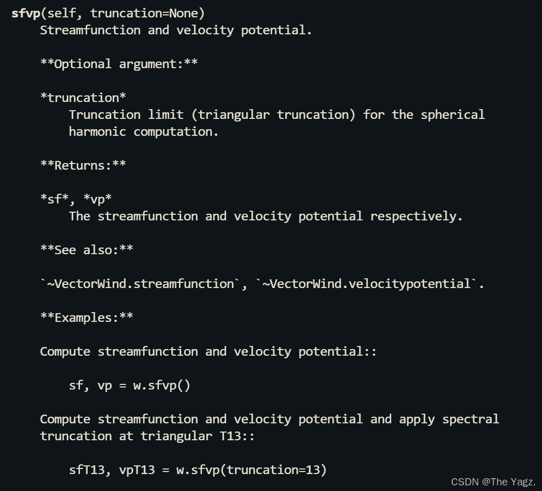
计算势函数（Velocity_Potential）的模块：

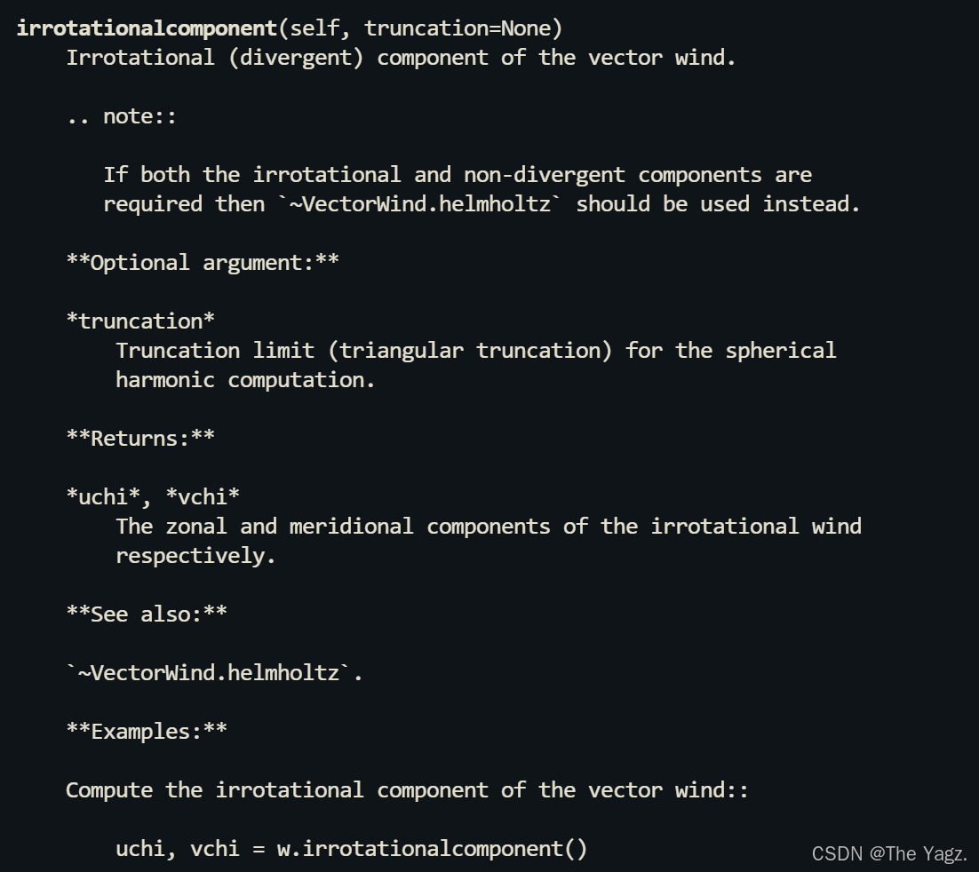
计算无旋风的模块：

计算

关键代码

w = VectorWind(uwnd, vwnd)
sf, vp = w.sfvp()
uchi, vchi = w.irrotationalcomponent()

本文代入的uwnd和vwnd都是二维的

官网案例

import cartopy.crs as ccrs
import matplotlib as mpl
import matplotlib.pyplot as plt
import xarray as xr

from windspharm.xarray import VectorWind
from windspharm.examples import example_data_path

mpl.rcParams['mathtext.default'] = 'regular'


# Read zonal and meridional wind components from file using the xarray module.
# The components are in separate files.
ds = xr.open_mfdataset([example_data_path(f)
                        for f in ('uwnd_mean.nc', 'vwnd_mean.nc')])
uwnd = ds['uwnd']
vwnd = ds['vwnd']

# Create a VectorWind instance to handle the computation of streamfunction and
# velocity potential.
w = VectorWind(uwnd, vwnd)

# Compute the streamfunction and velocity potential.
sf, vp = w.sfvp()

# Pick out the field for December.
sf_dec = sf[sf['time.month'] == 12]
vp_dec = vp[vp['time.month'] == 12]

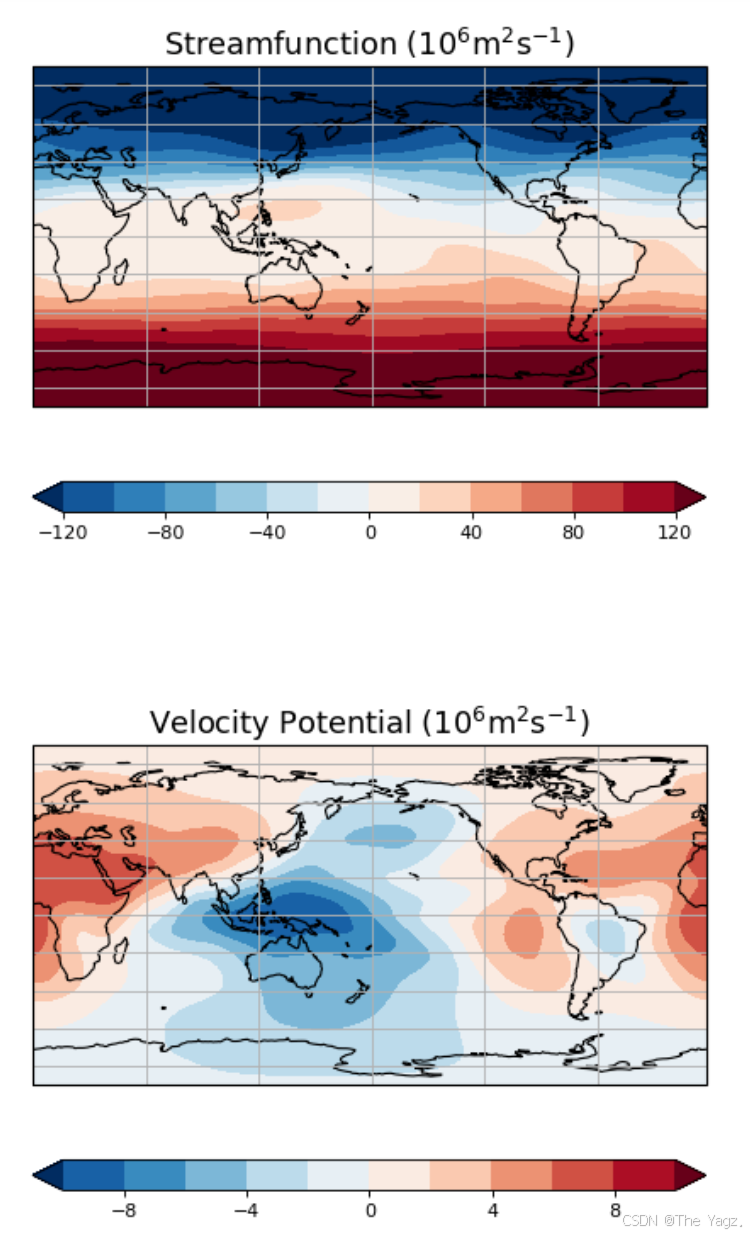
# Plot streamfunction.
clevs = [-120, -100, -80, -60, -40, -20, 0, 20, 40, 60, 80, 100, 120]
ax = plt.subplot(111, projection=ccrs.PlateCarree(central_longitude=180))
sf_dec *= 1e-6
fill_sf = sf_dec[0].plot.contourf(ax=ax, levels=clevs, cmap=plt.cm.RdBu_r,
                                  transform=ccrs.PlateCarree(), extend='both',
                                  add_colorbar=False)
ax.coastlines()
ax.gridlines()
plt.colorbar(fill_sf, orientation='horizontal')
plt.title('Streamfunction ($10^6$m$^2$s$^{-1}$)', fontsize=16)

# Plot velocity potential.
plt.figure()
clevs = [-10, -8, -6, -4, -2, 0, 2, 4, 6, 8, 10]
ax = plt.subplot(111, projection=ccrs.PlateCarree(central_longitude=180))
vp_dec *= 1e-6
fill_vp = vp_dec[0].plot.contourf(ax=ax, levels=clevs, cmap=plt.cm.RdBu_r,
                                  transform=ccrs.PlateCarree(), extend='both',
                                  add_colorbar=False)
ax.coastlines()
ax.gridlines()
plt.colorbar(fill_vp, orientation='horizontal')
plt.title('Velocity Potential ($10^6$m$^2$s$^{-1}$)', fontsize=16)
plt.show()

windspharm/examples/standard/sfvp_example.py at main · ajdawson/windspharm

结果

本人代码（仅参考）

from scipy.stats import pearsonr
from netCDF4 import Dataset#导入nc读取模块
from scipy.stats import linregress
import numpy as np
from windspharm.standard import VectorWind
from windspharm.tools import prep_data, recover_data, order_latdim

def pearsonr_calculate(RSEPD, data):
    # 获取数据的形状
    _, num_rows, num_cols = data.shape
    # 计算 Pearson 相关性
    r = np.zeros((num_rows, num_cols))
    p = np.zeros((num_rows, num_cols))
    for i in range(num_rows):
        for j in range(num_cols):
            r[i, j], p[i, j] = pearsonr(RSEPD, data[:, i, j])
    return r, p
def linregress_cal(RSEPD, data):
    # 获取数据的形状
    _, num_rows, num_cols = data.shape
    # 计算
    r = np.zeros((num_rows, num_cols))
    p = np.zeros((num_rows, num_cols))
    for i in range(num_rows):
        for j in range(num_cols):
            r[i, j], _, _, p[i, j], _ = linregress(RSEPD, data[:, i, j])
    return r, p
data1 = [-0.75026442, -0.86357667, -0.12060887, -0.23392112, -0.20452002, -1.31682566,
         1.7095556, 2.30981006, -0.94319569, 0.37062547, 1.11359328, 1.42842105,
         0.6015421, -1.0816169, 0.08949092, -0.59467469, -0.85070028, 0.17769421,
         -1.22003811, 0.37920974]
data2 = [1.08591854, -0.87351185, 0.2870476, -0.2542056, -1.64636511, -0.48580566,
         0.39111834, 1.55167779, -1.25865892, -0.09809948, 0.77882453, 1.08847766,
         1.39813079, -0.56129961, 0.59925984, -1.07653512, -0.19961111, -1.02449974,
         -1.28211749, 1.5802546]
data3 = [-1.39390487, -0.63518272, 0.37632011, 0.37670023, 0.12429967, -0.12810088,
         2.40008601, 1.13656274, -1.3908639, -0.1265804, 0.1265804, 1.13808323,
         -0.37822071, -0.88340194, -1.64136385, 1.13960371, -1.13504226, 0.88758328,
         0.12962137, -0.12277919]
data4 = [-1.1536111, -0.02746693, -1.09867723, -0.52187169, 1.1536111, -1.84028437,
         0.10986772, 1.7853505, 0.98880951, 1.01627644, 1.31841268, 0.52187169,
         0.27466931, -0.52187169, 1.1536111, -1.29094575, -0.16480159, 0.13733465,
         -1.20854496, -0.63173941]
testfile_path = '/data/ERA5_monthly/hgt/hgt2001.nc'  # 取个level
dataset = Dataset(testfile_path)
lats = dataset.variables['latitude'][:]
lons = dataset.variables['longitude'][:]

# 一些设置
z_path = '/data/ERA5_monthly/hgt/hgt'
u_path = '/data/ERA5_monthly/uwnd/uwnd'
v_path = '/data/ERA5_monthly/vwnd/vwnd'
w_path = '/data/ERA5_monthly/wwnd/wwnd'
star_year = 2001
end_year = 2020
RSEPD_v06 = [data2, data3, data4]
yearlis = range(star_year, end_year+1)
molis = ['June', 'July', 'August']
pressure_levels = [200, 500, 850]


for lev in range(len(pressure_levels)):
    for month in range(len(molis)):
        phi_data_years = np.zeros((len(yearlis), 181, 360))
        Uchi_data_years = np.zeros((len(yearlis), 181, 360))
        Vchi_data_years = np.zeros((len(yearlis), 181, 360))
        for year in yearlis:
            # 打开 u 和 v 的 NetCDF 文件
            f_u = Dataset(u_path + str(year) + '.nc', 'r')
            f_v = Dataset(v_path + str(year) + '.nc', 'r')
            level = f_u.variables['level'][:]
            lev_idx = np.where(level == pressure_levels[lev])[0][0]
            uwnd = f_u.variables['u'][month + 5, lev_idx, :, :]
            vwnd = f_v.variables['v'][month + 5, lev_idx, :, :]
            # 删除维度为1的坐标轴
            uwnd = np.squeeze(uwnd)
            vwnd = np.squeeze(vwnd)
            w = VectorWind(uwnd, vwnd)
            sf, vp = w.sfvp()
            uchi, vchi = w.irrotationalcomponent()
            phi_data_years[year - star_year, :, :] = np.array(vp).reshape(181, 360)
            Uchi_data_years[year - star_year, :, :] = np.array(uchi).reshape(181, 360)
            Vchi_data_years[year - star_year, :, :] = np.array(vchi).reshape(181, 360)
        r_w, p_w = linregress_cal(RSEPD_v06[month], phi_data_years)
        r_u, p_u = linregress_cal(RSEPD_v06[month], Uchi_data_years)
        r_v, p_v = linregress_cal(RSEPD_v06[month], Vchi_data_years)
        np.save('r_phi_' + str(pressure_levels[lev]) + '_' + molis[month] + '.npy', r_w)
        np.save('p_phi_' + str(pressure_levels[lev]) + '_' + molis[month] + '.npy', p_w)
        np.save('r_uchi_'+ str(pressure_levels[lev]) + '_' + molis[month] + '.npy', r_u)
        np.save('p_uchi_'+ str(pressure_levels[lev]) + '_' + molis[month] + '.npy', p_u)
        np.save('r_vchi_'+ str(pressure_levels[lev]) + '_' + molis[month] + '.npy', r_v)
        np.save('p_vchi_'+ str(pressure_levels[lev]) + '_' + molis[month] + '.npy', p_v)
    phi_data_years = np.zeros((len(yearlis), 181, 360))
    Uchi_data_years = np.zeros((len(yearlis), 181, 360))
    Vchi_data_years = np.zeros((len(yearlis), 181, 360))

    for year in yearlis:
        # 打开 u 和 v 的 NetCDF 文件
        f_u = Dataset(u_path + str(year) + '.nc', 'r')
        f_v = Dataset(v_path + str(year) + '.nc', 'r')
        level = f_u.variables['level'][:]
        lev_idx = np.where(level == pressure_levels[lev])[0][0]
        uwnd = f_u.variables['u'][5:8, lev_idx, :, :].mean(axis=0)
        vwnd = f_v.variables['v'][5:8, lev_idx, :, :].mean(axis=0)
        # 删除维度为1的坐标轴
        uwnd = np.squeeze(uwnd)
        vwnd = np.squeeze(vwnd)
        # 删除维度为1的坐标轴
        w = VectorWind(uwnd, vwnd)

        sf, vp = w.sfvp()
        uchi, vchi = w.irrotationalcomponent()

        phi_data_years[year - star_year, :, :] = np.array(vp).reshape(181, 360)
        Uchi_data_years[year - star_year, :, :] = np.array(uchi).reshape(181, 360)
        Vchi_data_years[year - star_year, :, :] = np.array(vchi).reshape(181, 360)
    r_w, p_w = linregress_cal(data1, phi_data_years)
    r_u, p_u = linregress_cal(data1, Uchi_data_years)
    r_v, p_v = linregress_cal(data1, Vchi_data_years)
    np.save('r_phi_' + str(pressure_levels[lev]) + '_summer.npy', r_w)
    np.save('p_phi_' + str(pressure_levels[lev]) + '_summer.npy', p_w)
    np.save('r_uchi_' + str(pressure_levels[lev]) + '_summer.npy', r_u)
    np.save('p_uchi_' + str(pressure_levels[lev]) + '_summer.npy', p_u)
    np.save('r_vchi_' + str(pressure_levels[lev]) + '_summer.npy', r_v)
    np.save('p_vchi_' + str(pressure_levels[lev]) + '_summer.npy', p_v)