Pandas+Matplotlib数据分析实践

最新推荐文章于 2024-03-12 21:15:38 发布

健康的码农

最新推荐文章于 2024-03-12 21:15:38 发布

阅读量8.4k

点赞数 2

文章标签： pandas matplotlib 数据分析

本文链接：https://blog.csdn.net/qq_52533648/article/details/131682285

版权

利用Python进行数据分析

1.MoviesLens 1M数据集

GroupLens实验室提供了一些从MoviesLens用户那里收集的20世纪90年代末到21世纪初的电影评分数据的集合。浙西额数据提供了电影的评分、流派、年份和观众数据（年龄、邮编、性别、职业）。
MovisLens1M数据集包含6000个用户对4000部电影的100万个评分。数据分布在三个表格之中：分别包含评分、用户信息和电影信息。

import pandas as pd

# 定义用户数据表的列名
unames = ["user_id", "gender", "age", "occupation", "zip"]
# 读取用户数据文件并创建数据帧（DataFrame）
users = pd.read_table("datasets/movielens/users.dat", sep="::",
                      header=None, names=unames, engine="python")

# 定义评分数据表的列名
rnames = ["user_id", "movie_id", "rating", "timestamp"]
# 读取评分数据文件并创建数据帧
ratings = pd.read_table("datasets/movielens/ratings.dat", sep="::",
                        header=None, names=rnames, engine="python")

# 定义电影数据表的列名
mnames = ["movie_id", "title", "genres"]
# 读取电影数据文件并创建数据帧
movies = pd.read_table("datasets/movielens/movies.dat", sep="::",
                       header=None, names=mnames, engine="python")

上面一段代码的功能是读取三个数据文件（users.dat、ratings.dat和movies.dat）的内容，并将它们存储在users、ratings和movies这三个数据中，以便后续进行数据分析和处理。

下面这段代码用于显示数据表的内容。使用head(5)方法可以显示数据表的前5行，这样可以快速查看数据的样本。而ratings数据表在末尾没有指定head(5)，因此将显示整个数据表。

# 输出users数据表的前5行
print(users.head(5))
print('==========================================')
# 输出ratings数据表的前5行
print(ratings.head(5))
print('==========================================')
# 输出movies数据表的前5行
print(movies.head(5))
print('===============================================================================')
# 输出ratings数据表的内容
print(ratings)

   user_id gender  age  occupation    zip
0        1      F    1          10  48067
1        2      M   56          16  70072
2        3      M   25          15  55117
3        4      M   45           7  02460
4        5      M   25          20  55455
==========================================
   user_id  movie_id  rating  timestamp
0        1      1193       5  978300760
1        1       661       3  978302109
2        1       914       3  978301968
3        1      3408       4  978300275
4        1      2355       5  978824291
==========================================
   movie_id                               title                        genres
0         1                    Toy Story (1995)   Animation|Children's|Comedy
1         2                      Jumanji (1995)  Adventure|Children's|Fantasy
2         3             Grumpier Old Men (1995)                Comedy|Romance
3         4            Waiting to Exhale (1995)                  Comedy|Drama
4         5  Father of the Bride Part II (1995)                        Comedy
===============================================================================
         user_id  movie_id  rating  timestamp
0              1      1193       5  978300760
1              1       661       3  978302109
2              1       914       3  978301968
3              1      3408       4  978300275
4              1      2355       5  978824291
...          ...       ...     ...        ...
1000204     6040      1091       1  956716541
1000205     6040      1094       5  956704887
1000206     6040       562       5  956704746
1000207     6040      1096       4  956715648
1000208     6040      1097       4  956715569

[1000209 rows x 4 columns]

下面这段代码使用了pd.merge()函数将ratings、users和movies数据表按照共同的列进行合并，生成了一个新的数据表data。合并的过程基于列名的匹配，将包含相同值的行进行连接。这样可以将用户信息、评分和电影信息整合在一个数据表中，方便进行综合分析和处理

# 使用pd.merge函数将ratings、users和movies数据表合并为一个新的数据表data
data = pd.merge(pd.merge(ratings, users), movies)

# 输出新数据表data的第一行
print(data.iloc[0])

# 输出新合并后的data数据表
data

user_id                                            1
movie_id                                        1193
rating                                             5
timestamp                                  978300760
gender                                             F
age                                                1
occupation                                        10
zip                                            48067
title         One Flew Over the Cuckoo's Nest (1975)
genres                                         Drama
Name: 0, dtype: object

	user_id	movie_id	rating	timestamp	gender	age	occupation	zip	title	genres
0	1	1193	5	978300760	F	1	10	48067	One Flew Over the Cuckoo's Nest (1975)	Drama
1	2	1193	5	978298413	M	56	16	70072	One Flew Over the Cuckoo's Nest (1975)	Drama
2	12	1193	4	978220179	M	25	12	32793	One Flew Over the Cuckoo's Nest (1975)	Drama
3	15	1193	4	978199279	M	25	7	22903	One Flew Over the Cuckoo's Nest (1975)	Drama
4	17	1193	5	978158471	M	50	1	95350	One Flew Over the Cuckoo's Nest (1975)	Drama
...	...	...	...	...	...	...	...	...	...	...
1000204	5949	2198	5	958846401	M	18	17	47901	Modulations (1998)	Documentary
1000205	5675	2703	3	976029116	M	35	14	30030	Broken Vessels (1998)	Drama
1000206	5780	2845	1	958153068	M	18	17	92886	White Boys (1999)	Drama
1000207	5851	3607	5	957756608	F	18	20	55410	One Little Indian (1973)	Comedy\|Drama\|Western
1000208	5938	2909	4	957273353	M	25	1	35401	Five Wives, Three Secretaries and Me (1998)	Documentary

1000209 rows × 10 columns

下面这段代码使用pivot_table()函数计算了按照电影标题（title）和性别（gender）分组的平均评分。rating为平均评分的值，index="title"指定电影标题为索引列，columns="gender"指定性别为列，aggfunc="mean"指定使用均值作为聚合函数

# 使用pivot_table函数计算平均评分，按照电影标题（title）作为索引，按照性别（gender）作为列，使用"rating"列的值进行计算
mean_ratings = data.pivot_table("rating", index="title", columns="gender", aggfunc="mean")

# 输出平均评分的前5行
mean_ratings.head(5)

gender	F	M
title
$1,000,000 Duck (1971)	3.375000	2.761905
'Night Mother (1986)	3.388889	3.352941
'Til There Was You (1997)	2.675676	2.733333
'burbs, The (1989)	2.793478	2.962085
...And Justice for All (1979)	3.828571	3.689024

下面这段代码的目的是根据评分数据表中的电影标题（title）进行分组，并计算每个电影标题的数量。使用groupby()函数按照标题进行分组，然后使用size()函数计算每个分组的大小，即对应标题的评分数量

# 使用groupby函数按照电影标题（title）进行分组，并计算每个标题的数量
ratings_by_title = data.groupby("title").size()

# 输出分组后的前几行结果
ratings_by_title.head()

# 通过筛选条件选取评分数量大于等于250的电影标题
active_titles = ratings_by_title.index[ratings_by_title >= 250]
active_titles

Index([''burbs, The (1989)', '10 Things I Hate About You (1999)',
       '101 Dalmatians (1961)', '101 Dalmatians (1996)', '12 Angry Men (1957)',
       '13th Warrior, The (1999)', '2 Days in the Valley (1996)',
       '20,000 Leagues Under the Sea (1954)', '2001: A Space Odyssey (1968)',
       '2010 (1984)',
       ...
       'X-Men (2000)', 'Year of Living Dangerously (1982)',
       'Yellow Submarine (1968)', 'You've Got Mail (1998)',
       'Young Frankenstein (1974)', 'Young Guns (1988)',
       'Young Guns II (1990)', 'Young Sherlock Holmes (1985)',
       'Zero Effect (1998)', 'eXistenZ (1999)'],
      dtype='object', name='title', length=1216)

下面这段代码使用active_titles列表中的活跃电影标题来筛选之前计算得到的平均评分数据表mean_ratings。

# 根据评分数量大于等于250的活跃电影标题筛选平均评分数据
mean_ratings = mean_ratings.loc[active_titles]

# 输出筛选后的平均评分数据
mean_ratings

gender	F	M
title
'burbs, The (1989)	2.793478	2.962085
10 Things I Hate About You (1999)	3.646552	3.311966
101 Dalmatians (1961)	3.791444	3.500000
101 Dalmatians (1996)	3.240000	2.911215
12 Angry Men (1957)	4.184397	4.328421
...	...	...
Young Guns (1988)	3.371795	3.425620
Young Guns II (1990)	2.934783	2.904025
Young Sherlock Holmes (1985)	3.514706	3.363344
Zero Effect (1998)	3.864407	3.723140
eXistenZ (1999)	3.098592	3.289086

1216 rows × 2 columns

这段代码对平均评分数据表mean_ratings中的索引进行重命名。其中，使用rename()方法将索引名从"Seven Samurai (The Magnificent Seven) (Shichinin no samurai) (1954)“修改为"Seven Samurai (Shichinin no samurai) (1954)”，以便更准确地表示电影的标题

# 重命名平均评分数据表中的索引（电影标题）
mean_ratings = mean_ratings.rename(index={"Seven Samurai (The Magnificent Seven) (Shichinin no samurai) (1954)":
                           "Seven Samurai (Shichinin no samurai) (1954)"})

# 按照女性观众（F）的评分降序排序
top_female_ratings = mean_ratings.sort_values("F", ascending=False)

# 输出女性观众评分最高的前几行
top_female_ratings.head()

gender	F	M
title
Close Shave, A (1995)	4.644444	4.473795
Wrong Trousers, The (1993)	4.588235	4.478261
Sunset Blvd. (a.k.a. Sunset Boulevard) (1950)	4.572650	4.464589
Wallace & Gromit: The Best of Aardman Animation (1996)	4.563107	4.385075
Schindler's List (1993)	4.562602	4.491415

这段代码计算了男性观众和女性观众评分之间的差异，并将结果存储在名为"diff"的新列中。通过计算"M"列（男性观众评分）减去"F"列（女性观众评分）得到评分差异值。

# 计算男性观众和女性观众评分的差异，并将结果存储在名为"diff"的新列中
mean_ratings["diff"] = mean_ratings["M"] - mean_ratings["F"]

# 按照差异值（diff）进行排序
sorted_by_diff = mean_ratings.sort_values("diff")

# 输出差异值最小的前几行
sorted_by_diff.head()

gender	F	M	diff
title
Dirty Dancing (1987)	3.790378	2.959596	-0.830782
Jumpin' Jack Flash (1986)	3.254717	2.578358	-0.676359
Grease (1978)	3.975265	3.367041	-0.608224
Little Women (1994)	3.870588	3.321739	-0.548849
Steel Magnolias (1989)	3.901734	3.365957	-0.535777

这段代码对差异值进行逆序排序，并使用[::-1]切片操作来反转排序顺序。然后，使用head()方法输出差异值最大的前几行结果。

# 对差异值进行逆序排序，并输出差异值最大的前几行
sorted_by_diff[::-1].head()

gender	F	M	diff
title
Good, The Bad and The Ugly, The (1966)	3.494949	4.221300	0.726351
Kentucky Fried Movie, The (1977)	2.878788	3.555147	0.676359
Dumb & Dumber (1994)	2.697987	3.336595	0.638608
Longest Day, The (1962)	3.411765	4.031447	0.619682
Cable Guy, The (1996)	2.250000	2.863787	0.613787

这段代码使用groupby()函数按照电影标题（title）进行分组，并计算每个标题对应的评分标准差。通过指定[“rating”]来选择需要计算标准差的列。
接下来，代码使用之前筛选出的活跃电影标题active_titles来筛选评分标准差数据。

# 使用groupby函数按照电影标题（title）进行分组，并计算每个标题对应的评分标准差
rating_std_by_title = data.groupby("title")["rating"].std()

# 根据评分数量大于等于250的活跃电影标题筛选评分标准差数据
rating_std_by_title = rating_std_by_title.loc[active_titles]

# 输出筛选后的评分标准差数据的前几行
rating_std_by_title.head()

title
'burbs, The (1989)                   1.107760
10 Things I Hate About You (1999)    0.989815
101 Dalmatians (1961)                0.982103
101 Dalmatians (1996)                1.098717
12 Angry Men (1957)                  0.812731
Name: rating, dtype: float64

这段代码对评分标准差数据进行降序排序，并使用切片操作[:10]选择前10个结果进行输出。

# 对评分标准差数据进行降序排序，并输出前10个结果
rating_std_by_title.sort_values(ascending=False)[:10]

title
Dumb & Dumber (1994)                     1.321333
Blair Witch Project, The (1999)          1.316368
Natural Born Killers (1994)              1.307198
Tank Girl (1995)                         1.277695
Rocky Horror Picture Show, The (1975)    1.260177
Eyes Wide Shut (1999)                    1.259624
Evita (1996)                             1.253631
Billy Madison (1995)                     1.249970
Fear and Loathing in Las Vegas (1998)    1.246408
Bicentennial Man (1999)                  1.245533
Name: rating, dtype: float64

这段代码用于处理电影数据表中的"genres"列，进行拆分和重命名列的操作。

# 输出电影数据表中"genres"列的前几行内容
movies["genres"].head()

# 使用str.split("|")方法将"genres"列中的多个流派以"|"进行拆分
movies["genres"].head().str.split("|")

# 将拆分后的流派存储在名为"genre"的新列中
movies["genre"] = movies.pop("genres").str.split("|")

# 输出更新后的电影数据表
movies.head()

	movie_id	title	genre
0	1	Toy Story (1995)	[Animation, Children's, Comedy]
1	2	Jumanji (1995)	[Adventure, Children's, Fantasy]
2	3	Grumpier Old Men (1995)	[Comedy, Romance]
3	4	Waiting to Exhale (1995)	[Comedy, Drama]
4	5	Father of the Bride Part II (1995)	[Comedy]

这段代码使用explode()方法根据"genre"列展开电影数据表，即将多个流派的项拆分为单独的行，以展示每个电影与其对应的单个流派的关系。

# 使用explode方法根据"genre"列展开电影数据表
movies_exploded = movies.explode("genre")

# 输出展开后的前10行结果
movies_exploded[:10]

	movie_id	title	genre
0	1	Toy Story (1995)	Animation
0	1	Toy Story (1995)	Children's
0	1	Toy Story (1995)	Comedy
1	2	Jumanji (1995)	Adventure
1	2	Jumanji (1995)	Children's
1	2	Jumanji (1995)	Fantasy
2	3	Grumpier Old Men (1995)	Comedy
2	3	Grumpier Old Men (1995)	Romance
3	4	Waiting to Exhale (1995)	Comedy
3	4	Waiting to Exhale (1995)	Drama

下面使用pd.merge()函数将展开后的电影数据表movies_exploded与ratings和users数据表进行合并，生成合并后的数据表ratings_with_genre。
输出合并后的数据表ratings_with_genre的第一行，使用iloc[0]来获取第一行的内容。
使用groupby()函数按照流派和年龄进行分组，计算评分的均值，并使用unstack(“age”)将年龄作为列展开，生成了以流派为行、年龄为列的评分均值数据表genre_ratings。
输出按照流派和年龄分组后的评分均值数据表的前10行

# 使用pd.merge函数将展开后的电影数据表movies_exploded与ratings和users数据表合并
ratings_with_genre = pd.merge(pd.merge(movies_exploded, ratings), users)

# 输出合并后的数据表ratings_with_genre的第一行
ratings_with_genre.iloc[0]

# 使用groupby函数按照流派和年龄分组，计算评分的均值，并将结果以年龄为列展开
genre_ratings = (ratings_with_genre.groupby(["genre", "age"])
                 ["rating"].mean()
                 .unstack("age"))

# 输出按照流派和年龄分组后的评分均值的前10行
genre_ratings[:10]

age	1	18	25	35	45	50	56
genre
Action	3.506385	3.447097	3.453358	3.538107	3.528543	3.611333	3.610709
Adventure	3.449975	3.408525	3.443163	3.515291	3.528963	3.628163	3.649064
Animation	3.476113	3.624014	3.701228	3.740545	3.734856	3.780020	3.756233
Children's	3.241642	3.294257	3.426873	3.518423	3.527593	3.556555	3.621822
Comedy	3.497491	3.460417	3.490385	3.561984	3.591789	3.646868	3.650949
Crime	3.710170	3.668054	3.680321	3.733736	3.750661	3.810688	3.832549
Documentary	3.730769	3.865865	3.946690	3.953747	3.966521	3.908108	3.961538
Drama	3.794735	3.721930	3.726428	3.782512	3.784356	3.878415	3.933465
Fantasy	3.317647	3.353778	3.452484	3.482301	3.532468	3.581570	3.532700
Film-Noir	4.145455	3.997368	4.058725	4.064910	4.105376	4.175401	4.125932

2.美国1880-2010年的婴儿名字

美国社会保障局（SSA）提供了从1880年至现在的婴儿姓名频率的数据。可以使用这些数据做很多事情：
根据给定的名字对婴儿名字随时间的比例进行可视化
确定一个名字的相对排位
确定每年最受欢迎的名字，或者流行程度最高或最低的名字

#!head -n 10 datasets/babynames/yob1880.txt

我们开始读取并加载"yob1880.txt"文件，该文件包含了1880年的婴儿姓名频率数据。通过使用Pandas库中的函数和数据结构，我们可以轻松地读取、处理和分析这些数据。

# 导入所需的库
import pandas as pd

# 读取名为"yob1880.txt"的文件，并将数据存储到DataFrame对象names1880中
names1880 = pd.read_csv("datasets/babynames/yob1880.txt", names=["name", "sex", "births"])

# 输出names1880，查看读取的数据
names1880

	name	sex	births
0	Mary	F	7065
1	Anna	F	2604
2	Emma	F	2003
3	Elizabeth	F	1939
4	Minnie	F	1746
...	...	...	...
1995	Woodie	M	5
1996	Worthy	M	5
1997	Wright	M	5
1998	York	M	5
1999	Zachariah	M	5

2000 rows × 3 columns

# 对性别进行分组，并计算每个性别的出生次数总和
names1880.groupby("sex")["births"].sum()

sex
F     90993
M    110493
Name: births, dtype: int64

这段代码的目的是将从1880年到2010年的婴儿姓名频率数据读取为多个数据块，并将它们连接成一个单一的DataFrame对象。通过使用循环迭代和pd.concat()函数，每个年份的数据被读取为一个DataFrame，并添加了表示年份的列。然后，这些数据块被添加到列表中，并使用pd.concat()函数进行连接，最终形成一个包含所有年份的数据的DataFrame对象。

# 创建一个空列表用于存储数据分块
pieces = []

# 循环迭代从1880年到2010年（不包括2011年）
for year in range(1880, 2011):
    # 根据年份构建文件路径
    path = f"datasets/babynames/yob{year}.txt"

    # 读取文件数据，并指定列名为["name", "sex", "births"]
    frame = pd.read_csv(path, names=["name", "sex", "births"])

    # 添加一个表示年份的列
    frame["year"] = year

    # 将每个年份的数据块添加到列表中
    pieces.append(frame)

# 将所有数据块连接成一个单一的DataFrame
names = pd.concat(pieces, ignore_index=True)
names

	name	sex	births	year
0	Mary	F	7065	1880
1	Anna	F	2604	1880
2	Emma	F	2003	1880
3	Elizabeth	F	1939	1880
4	Minnie	F	1746	1880
...	...	...	...	...
1690779	Zymaire	M	5	2010
1690780	Zyonne	M	5	2010
1690781	Zyquarius	M	5	2010
1690782	Zyran	M	5	2010
1690783	Zzyzx	M	5	2010

1690784 rows × 4 columns

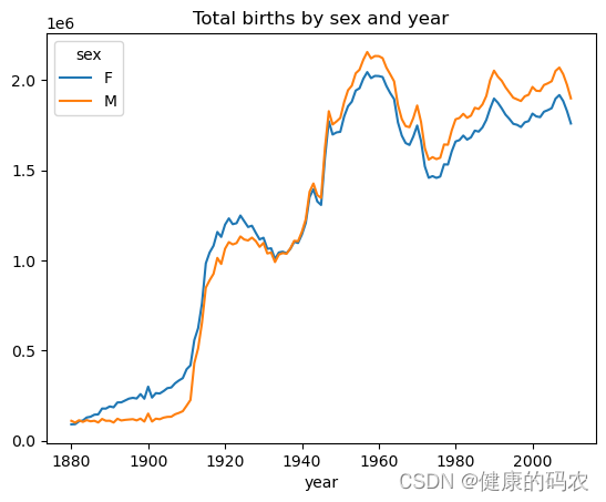
这段代码的目的是计算并可视化每年每个性别的总出生数。通过使用pivot_table函数，我们根据年份和性别对数据进行汇总，并计算每年每个性别的出生总数。然后，我们使用tail()函数查看最后几行透视表的数据，以确保计算正确。最后，使用plot函数绘制总出生数随年份和性别变化的图表，并添加标题以描述图表内容。

# 根据年份和性别计算出生总数的透视表
total_births = names.pivot_table("births", index="year", columns="sex", aggfunc=sum)

# 输出透视表的最后几行数据
total_births.tail()

# 绘制以年份和性别为横纵轴的总出生数图表
total_births.plot(title="Total births by sex and year")

<Axes: title={'center': 'Total births by sex and year'}, xlabel='year'>

在这里插入图片描述

这段代码的目的是计算每个婴儿姓名在其所在组中的比例，并将比例值添加为新的列"prop"。通过使用groupby函数将数据按照"year"和"sex"进行分组，然后应用add_prop函数来计算比例并添加到每个组的DataFrame中。最后，将经过处理后的DataFrame赋值给names变量，并输出结果。

# 定义一个函数用于添加比例列
def add_prop(group):
    group["prop"] = group["births"] / group["births"].sum()
    return group

# 对names DataFrame按照"year"和"sex"进行分组，并对每个组应用add_prop函数
names = names.groupby(["year", "sex"], group_keys=False).apply(add_prop)

# 输出经过处理后的names DataFrame
names

	name	sex	births	year	prop
0	Mary	F	7065	1880	0.077643
1	Anna	F	2604	1880	0.028618
2	Emma	F	2003	1880	0.022013
3	Elizabeth	F	1939	1880	0.021309
4	Minnie	F	1746	1880	0.019188
...	...	...	...	...	...
1690779	Zymaire	M	5	2010	0.000003
1690780	Zyonne	M	5	2010	0.000003
1690781	Zyquarius	M	5	2010	0.000003
1690782	Zyran	M	5	2010	0.000003
1690783	Zzyzx	M	5	2010	0.000003

1690784 rows × 5 columns

# 按年份和性别分组，并计算比例列的总和
names.groupby(["year", "sex"])["prop"].sum()

year  sex
1880  F      1.0
      M      1.0
1881  F      1.0
      M      1.0
1882  F      1.0
            ... 
2008  M      1.0
2009  F      1.0
      M      1.0
2010  F      1.0
      M      1.0
Name: prop, Length: 262, dtype: float64

这段代码的目的是对按照年份和性别分组的names DataFrame，获取每个组中出生次数前1000名的数据。通过使用groupby函数按照"year"和"sex"对数据进行分组，然后对每个组应用get_top1000函数，将每个组中出生次数前1000名的数据提取出来。最后，输出获取到的出生次数前1000名的数据的前几行。

# 定义一个函数用于获取每个组中出生次数前1000名的数据
def get_top1000(group):
    return group.sort_values("births", ascending=False)[:1000]

# 对names DataFrame按照"year"和"sex"进行分组
grouped = names.groupby(["year", "sex"])

# 对每个组应用get_top1000函数，获取出生次数前1000名的数据
top1000 = grouped.apply(get_top1000)

# 输出获取到的出生次数前1000名的数据的前几行
top1000.head()

			name	sex	births	year	prop
year	sex
1880	F	0	Mary	F	7065	1880	0.077643
		1	Anna	F	2604	1880	0.028618
		2	Emma	F	2003	1880	0.022013
		3	Elizabeth	F	1939	1880	0.021309
		4	Minnie	F	1746	1880	0.019188

这段代码的目的是重置top1000 DataFrame的索引，去除之前的分组索引，并生成默认的数值索引。通过使用reset_index函数，我们可以重新设置DataFrame的索引，以便更好地进行后续的数据处理和分析。最后，输出重置索引后的DataFrame的前几行数据。

# 重置索引，去除之前的分组索引
top1000 = top1000.reset_index(drop=True)

# 输出重置索引后的前几行数据
top1000.head()

	name	sex	births	year	prop
0	Mary	F	7065	1880	0.077643
1	Anna	F	2604	1880	0.028618
2	Emma	F	2003	1880	0.022013
3	Elizabeth	F	1939	1880	0.021309
4	Minnie	F	1746	1880	0.019188

这段代码的目的是根据性别和特定姓名，从top1000 DataFrame中提取数据，并进行进一步的分析和可视化。首先，我们根据性别筛选出男孩和女孩的数据，分别存储在boys和girls变量中。然后，我们使用pivot_table函数根据年份和姓名计算出生次数的透视表，存储在total_births变量中，并输出其基本信息。接下来，我们从透视表中选择特定的姓名列，即"John"、“Harry”、"Mary"和"Marilyn"列，并将结果存储在subset变量中。最后，使用plot函数绘制子图，显示每个姓名的每年出生次数。

# 从top1000中筛选出性别为男孩的数据
boys = top1000[top1000["sex"] == "M"]

# 从top1000中筛选出性别为女孩的数据
girls = top1000[top1000["sex"] == "F"]

# 根据年份和姓名计算出生次数的透视表
total_births = top1000.pivot_table("births", index="year", columns="name", aggfunc=sum)

# 输出透视表的基本信息
total_births.info()

# 从透视表中选择特定的姓名列
subset = total_births[["John", "Harry", "Mary", "Marilyn"]]

# 绘制子图，显示每个姓名的每年出生次数
subset.plot(subplots=True, figsize=(12, 10), title="Number of births per year")

<class 'pandas.core.frame.DataFrame'>
Index: 131 entries, 1880 to 2010
Columns: 6868 entries, Aaden to Zuri
dtypes: float64(6868)
memory usage: 6.9 MB


array([<Axes: xlabel='year'>, <Axes: xlabel='year'>,
       <Axes: xlabel='year'>, <Axes: xlabel='year'>], dtype=object)

在这里插入图片描述

这段代码的目的是根据年份和性别计算比例，并将比例的总和可视化为图表。通过使用pivot_table函数，我们计算了每个年份和性别的比例总和，并将结果存储在table变量中。然后，使用plot函数绘制以年份和性别为横纵轴的比例总和图表，并添加标题和自定义的y轴刻度。

import numpy as np
# 根据年份和性别计算比例的透视表
table = top1000.pivot_table("prop", index="year", columns="sex", aggfunc=sum)

# 绘制以年份和性别为横纵轴的比例总和图表
table.plot(title="Sum of top1000.prop by year and sex", yticks=np.linspace(0, 1.2, 13))

<Axes: title={'center': 'Sum of top1000.prop by year and sex'}, xlabel='year'>

在这里插入图片描述

这段代码的目的是从boys DataFrame中筛选出年份为2010的数据，并将结果存储在df变量中。最后，输出筛选后的数据。这可以用于查看特定年份的男孩数据。

# 从boys DataFrame中筛选出年份为2010的数据
df = boys[boys["year"] == 2010]

# 输出筛选后的数据
df

	name	sex	births	year	prop
260877	Jacob	M	21875	2010	0.011523
260878	Ethan	M	17866	2010	0.009411
260879	Michael	M	17133	2010	0.009025
260880	Jayden	M	17030	2010	0.008971
260881	William	M	16870	2010	0.008887
...	...	...	...	...	...
261872	Camilo	M	194	2010	0.000102
261873	Destin	M	194	2010	0.000102
261874	Jaquan	M	194	2010	0.000102
261875	Jaydan	M	194	2010	0.000102
261876	Maxton	M	193	2010	0.000102

1000 rows × 5 columns

这段代码的目的是对df DataFrame中的"prop"列进行操作，计算累积和并寻找特定条件下的位置。首先，对"prop"列进行降序排序，并计算累积和，得到累积和的结果存储在prop_cumsum变量中。然后，输出累积和的前10个值。最后，使用searchsorted函数在累积和中寻找第一个超过0.5的位置。这些操作可以用于分析累积概率和找到特定阈值的位置。

# 对df中的"prop"列按降序排序，并计算累积和
prop_cumsum = df["prop"].sort_values(ascending=False).cumsum()

# 输出累积和的前10个值
prop_cumsum[:10]

# 寻找累积和超过0.5的位置
prop_cumsum.searchsorted(0.5)

这段代码的目的是针对年份为1900的男孩数据进行分析。首先，从boys DataFrame中筛选出年份为1900的数据，存储在df变量中。然后，对筛选后的数据按照"prop"列进行降序排序，并计算累积和，结果存储在in1900变量中。最后，使用searchsorted函数寻找累积和超过0.5的位置，并将结果加1得到排名。这个分析可以用于确定在1900年出生的男孩名字中，占据前50%累积概率的排名。

# 从boys DataFrame中筛选出年份为1900的数据
df = boys[boys.year == 1900]

# 对筛选后的数据按"prop"列降序排序，并计算累积和
in1900 = df.sort_values("prop", ascending=False).prop.cumsum()

# 寻找累积和超过0.5的位置，并加上1得到排名
in1900.searchsorted(0.5) + 1

这段代码的目的是计算每个年份和性别组合中，累积概率超过指定阈值的排名。首先，定义了一个函数get_quantile_count，用于计算累积概率超过指定阈值的排名。然后，使用groupby函数按照"year"和"sex"对数据进行分组，对每个组应用get_quantile_count函数，计算累积概率超过指定阈值的排名，并将结果存储在diversity变量中。最后，通过unstack函数将结果重新排列成二维表格形式。

# 定义一个函数用于计算累积概率超过指定阈值的排名
def get_quantile_count(group, q=0.5):
    group = group.sort_values("prop", ascending=False)
    return group.prop.cumsum().searchsorted(q) + 1

# 按年份和性别分组，对每个组应用get_quantile_count函数，计算累积概率超过指定阈值的排名
diversity = top1000.groupby(["year", "sex"]).apply(get_quantile_count)

# 将结果重新排列成二维表格形式
diversity = diversity.unstack()

# 输出多样性数据的前几行
diversity.head()

# 绘制每个年份和性别组合中的流行姓名数量图表
diversity.plot(title="Number of popular names in top 50%")

<Axes: title={'center': 'Number of popular names in top 50%'}, xlabel='year'>

在这里插入图片描述

这段代码的目的是根据名字的最后一个字母、性别和年份计算出生次数，并选择特定的年份列进行分析。首先，定义了一个函数get_last_letter，用于从名字中获取最后一个字母。然后，通过map函数将names DataFrame中的每个名字映射到其最后一个字母，结果存储在last_letters变量中。修改映射结果的列名为"last_letter"。接下来，使用pivot_table函数根据最后一个字母、性别和年份计算出生次数的透视表，将结果存储在table变量中。然后，从透视表中选择特定的年份列，并重新排序为[1910, 1960, 2010]，将结果存储在subtable变量中。最后，输出选择的列的前几行数据。这个分析可以用于观察不同年份、性别和名字最后一个字母之间的出生次数变化。

# 定义一个函数用于获取名字的最后一个字母
def get_last_letter(x):
    return x[-1]

# 将名字列中的每个名字映射到其最后一个字母
last_letters = names["name"].map(get_last_letter)

# 修改映射结果的列名为"last_letter"
last_letters.name = "last_letter"

# 根据最后一个字母和性别、年份计算出生次数的透视表
table = names.pivot_table("births", index=last_letters, columns=["sex", "year"], aggfunc=sum)

# 从透视表中选择特定的年份列，并重新排序
subtable = table.reindex(columns=[1910, 1960, 2010], level="year")

# 输出选择的列的前几行数据
subtable.head()

sex	F			M
year	1910	1960	2010	1910	1960	2010
last_letter
a	108376.0	691247.0	670605.0	977.0	5204.0	28438.0
b	NaN	694.0	450.0	411.0	3912.0	38859.0
c	5.0	49.0	946.0	482.0	15476.0	23125.0
d	6750.0	3729.0	2607.0	22111.0	262112.0	44398.0
e	133569.0	435013.0	313833.0	28655.0	178823.0	129012.0

这段代码的目的是计算每个元素在列总和中的比例，即每个元素在对应列的出生次数中所占比例。首先，通过对subtable中的列进行求和，计算各列的总和，存储在column_sum变量中。然后，将subtable中的每个元素除以对应列总和的值，得到比例表，将结果存储在letter_prop变量中。最后，输出比例表，展示每个元素在对应列总和中的比例。

# 按列对数据进行求和，计算各列的总和
column_sum = subtable.sum()

# 计算每个元素在列总和中的比例
letter_prop = subtable / column_sum

# 输出比例表
letter_prop

sex	F			M
year	1910	1960	2010	1910	1960	2010
last_letter
a	0.273390	0.341853	0.381240	0.005031	0.002440	0.014980
b	NaN	0.000343	0.000256	0.002116	0.001834	0.020470
c	0.000013	0.000024	0.000538	0.002482	0.007257	0.012181
d	0.017028	0.001844	0.001482	0.113858	0.122908	0.023387
e	0.336941	0.215133	0.178415	0.147556	0.083853	0.067959
f	NaN	0.000010	0.000055	0.000783	0.004325	0.001188
g	0.000144	0.000157	0.000374	0.002250	0.009488	0.001404
h	0.051529	0.036224	0.075852	0.045562	0.037907	0.051670
i	0.001526	0.039965	0.031734	0.000844	0.000603	0.022628
j	NaN	NaN	0.000090	NaN	NaN	0.000769
k	0.000121	0.000156	0.000356	0.036581	0.049384	0.018541
l	0.043189	0.033867	0.026356	0.065016	0.104904	0.070367
m	0.001201	0.008613	0.002588	0.058044	0.033827	0.024657
n	0.079240	0.130687	0.140210	0.143415	0.152522	0.362771
o	0.001660	0.002439	0.001243	0.017065	0.012829	0.042681
p	0.000018	0.000023	0.000020	0.003172	0.005675	0.001269
q	NaN	NaN	0.000030	NaN	NaN	0.000180
r	0.013390	0.006764	0.018025	0.064481	0.031034	0.087477
s	0.039042	0.012764	0.013332	0.130815	0.102730	0.065145
t	0.027438	0.015201	0.007830	0.072879	0.065655	0.022861
u	0.000684	0.000574	0.000417	0.000124	0.000057	0.001221
v	NaN	0.000060	0.000117	0.000113	0.000037	0.001434
w	0.000020	0.000031	0.001182	0.006329	0.007711	0.016148
x	0.000015	0.000037	0.000727	0.003965	0.001851	0.008614
y	0.110972	0.152569	0.116828	0.077349	0.160987	0.058168
z	0.002439	0.000659	0.000704	0.000170	0.000184	0.001831

这段代码的目的是绘制男孩和女孩每个字母在不同年份中的比例条形图，并在每个子图中添加相应的标题。通过使用plot函数和指定的绘图类型（条形图），我们可以可视化每个字母在男孩和女孩中的相对流行程度。

import matplotlib.pyplot as plt

# 创建包含两个子图的图形
fig, axes = plt.subplots(2, 1, figsize=(10, 8))

# 在第一个子图中绘制男孩的比例条形图
letter_prop["M"].plot(kind="bar", rot=0, ax=axes[0], title="Male")

# 在第二个子图中绘制女孩的比例条形图
letter_prop["F"].plot(kind="bar", rot=0, ax=axes[1], title="Female", legend=False)

<Axes: title={'center': 'Female'}, xlabel='last_letter'>

在这里插入图片描述

这段代码的目的是计算每个字母在男孩和女孩中的相对流行程度，并选择特定字母在男孩中的比例进行进一步分析。首先，通过plt.subplots_adjust函数调整子图之间的垂直间距，以提高图表的可读性。然后，计算每个元素在透视表总和中的比例，即每个字母在男孩和女孩中的相对流行程度，结果存储在letter_prop变量中。接下来，从比例表中选择字母为"d"、"n"和"y"在男孩中的比例，并进行转置操作，将结果存储在dny_ts变量中。最后，输出选择的数据的前几行，用于查看分析结果

# 调整子图之间的垂直间距
plt.subplots_adjust(hspace=0.25)

# 计算每个元素在透视表总和中的比例
letter_prop = table / table.sum()

# 选择特定字母（"d", "n", "y"）在男孩中的比例，并进行转置
dny_ts = letter_prop.loc[["d", "n", "y"], "M"].T

# 输出选择的数据的前几行
dny_ts.head()

last_letter	d	n	y
year
1880	0.083055	0.153213	0.075760
1881	0.083247	0.153214	0.077451
1882	0.085340	0.149560	0.077537
1883	0.084066	0.151646	0.079144
1884	0.086120	0.149915	0.080405

<Figure size 640x480 with 0 Axes>

这段代码的目的是关闭之前创建的所有图形，并创建一个新的图形对象。然后，使用plot函数在新的图形中绘制dny_ts数据。

# 关闭所有之前创建的图形
plt.close("all")

# 创建一个新的图形
fig = plt.figure()

# 在新图形中绘制dny_ts数据
dny_ts.plot()

<Axes: xlabel='year'>




<Figure size 640x480 with 0 Axes>

在这里插入图片描述

这段代码的目的是筛选出在top1000中包含"Lesl"的名字。首先，使用pd.Series函数创建一个包含top1000中所有不重复名字的Series，存储在all_names变量中。然后，使用str.contains方法筛选出包含"Lesl"的名字，并将结果存储在lesley_like变量中。最后，输出筛选结果，显示包含"Lesl"的名字列表。

# 创建一个包含top1000中所有不重复名字的Series
all_names = pd.Series(top1000["name"].unique())

# 从所有名字中筛选出包含"Lesl"的名字
lesley_like = all_names[all_names.str.contains("Lesl")]

# 输出筛选结果
lesley_like

632     Leslie
2294    Lesley
4262    Leslee
4728     Lesli
6103     Lesly
dtype: object

这段代码的目的是从top1000中筛选出包含在lesley_like中的数据，并计算每个名字的总出生次数。最后，输出每个名字的总出生次数。

# 从top1000中筛选出包含在lesley_like中的数据
filtered = top1000[top1000["name"].isin(lesley_like)]

# 按名字分组，计算每个名字的总出生次数
filtered.groupby("name")["births"].sum()

name
Leslee      1082
Lesley     35022
Lesli        929
Leslie    370429
Lesly      10067
Name: births, dtype: int64

这段代码的目的是根据筛选后的数据，计算每个年份中男孩和女孩的比例。首先，使用pivot_table函数根据年份和性别对筛选后的数据进行透视，计算每个年份中男孩和女孩的出生次数总和，结果存储在table中。然后，使用div函数计算每个年份中男孩和女孩的比例，即每个性别在总出生次数中的占比。最后，输出计算后的比例表的最后几行数据，用于观察男孩和女孩的比例随年份变化的趋势

# 根据年份、性别对筛选后的数据进行透视，计算出生次数的总和
table = filtered.pivot_table("births", index="year", columns="sex", aggfunc="sum")

# 计算每个年份中男孩和女孩的比例
table = table.div(table.sum(axis="columns"), axis="index")

# 输出计算后的比例表
table.tail()

sex	F	M
year
2006	1.0	NaN
2007	1.0	NaN
2008	1.0	NaN
2009	1.0	NaN
2010	1.0	NaN

这段代码的目的是在新的图形中绘制男孩和女孩的比例曲线。首先，创建一个新的图形对象。然后，使用plot函数绘制男孩和女孩的比例曲线，通过style参数指定男孩曲线的样式为黑色实线，女孩曲线的样式为黑色虚线。通过观察曲线的变化，可以了解男孩和女孩在不同年份中的出生比例变化情况。

# 创建一个新的图形对象
fig = plt.figure()

# 在新图形中绘制男孩和女孩的比例曲线
table.plot(style={"M": "k-", "F": "k--"})

<Axes: xlabel='year'>




<Figure size 640x480 with 0 Axes>

在这里插入图片描述

3.美国农业部视频数据库

美国农业部提供了食物营养信息数据库。每种事务都有一些识别属性以及两份营养元素和营养比例的列表。这种形式的数据不适合分析，所以需要做一些工作将数据转换成更好的形式。

这段代码的目的是从指定的JSON文件加载数据，并计算数据中的记录数量。最后，输出记录数量。这个步骤有助于我们了解数据的规模和总体结构。

import json

# 从JSON文件加载数据
db = json.load(open("datasets/usda_food/database.json"))

# 计算数据中的记录数量
record_count = len(db)

# 输出记录数量
record_count

这段代码的目的是获取数据中第一个记录的键值，获取第一个记录中"nutrients"键的第一个元素，创建一个DataFrame来存储"nutrients"中的数据，并输出前7行的数据。这些步骤有助于我们了解数据的结构和内容。

# 获取第一个记录的键值
db[0].keys()

# 获取第一个记录中的"nutrients"键的第一个元素
db[0]["nutrients"][0]

# 创建一个DataFrame来存储"nutrients"中的数据
nutrients = pd.DataFrame(db[0]["nutrients"])

# 输出前7行的数据
nutrients.head(7)

	value	units	description	group
0	25.18	g	Protein	Composition
1	29.20	g	Total lipid (fat)	Composition
2	3.06	g	Carbohydrate, by difference	Composition
3	3.28	g	Ash	Other
4	376.00	kcal	Energy	Energy
5	39.28	g	Water	Composition
6	1573.00	kJ	Energy	Energy

这段代码的目的是从数据中提取指定键名的数据，并创建一个DataFrame来存储提取的键值数据。然后，输出DataFrame的前几行数据和基本信息。通过这些步骤，我们可以了解数据中的描述、分组、ID和制造商等关键信息，并对数据的基本结构有一个初步的了解

# 定义需要提取的键名列表
info_keys = ["description", "group", "id", "manufacturer"]

# 创建一个DataFrame来存储提取的键值数据
info = pd.DataFrame(db, columns=info_keys)

# 输出DataFrame的前几行数据
info.head()

# 输出DataFrame的基本信息
info.info()

<class 'pandas.core.frame.DataFrame'>
RangeIndex: 6636 entries, 0 to 6635
Data columns (total 4 columns):
 #   Column        Non-Null Count  Dtype 
---  ------        --------------  ----- 
 0   description   6636 non-null   object
 1   group         6636 non-null   object
 2   id            6636 non-null   int64 
 3   manufacturer  5195 non-null   object
dtypes: int64(1), object(3)
memory usage: 207.5+ KB

这行代码使用 pd.value_counts() 函数对 info 数据框中的 “group” 列进行计数，然后使用 [:10] 索引选取前10个值。这行代码的目的是统计 info 数据框中 “group” 列中出现次数最多的10个值。

# 对 info 数据框中的 "group" 列进行计数，选取前10个值
pd.value_counts(info["group"])[:10]

group
Vegetables and Vegetable Products    812
Beef Products                        618
Baked Products                       496
Breakfast Cereals                    403
Legumes and Legume Products          365
Fast Foods                           365
Lamb, Veal, and Game Products        345
Sweets                               341
Fruits and Fruit Juices              328
Pork Products                        328
Name: count, dtype: int64

# 对 info 数据框中的 "group" 列进行计数，选取前10个值
top_10 = pd.value_counts(info["group"])[:10]

# 绘制条形图可视化结果
top_10.plot(kind='bar')

<Axes: xlabel='group'>

在这里插入图片描述

这段代码的目的是将 db 中的数据转换为一个更适合分析的形式。首先，创建一个空列表 nutrients 用于存储转换后的数据。然后，使用 for 循环遍历 db 中的每一条记录。对于每一条记录，使用 pd.DataFrame() 函数将其 “nutrients” 列转换为一个数据框 fnuts，并在 fnuts 中添加一列 “id”，其值为当前记录的 “id” 值。最后，将 fnuts 添加到 nutrients 列表中。
在完成遍历后，使用 pd.concat() 函数将 nutrients 列表中的所有数据框合并为一个大的数据框 nutrients，并使用 ignore_index=True 参数重置索引。

# 创建空列表用于存储转换后的数据
nutrients = []

# 遍历 db 中的每一条记录
for rec in db:
    # 将当前记录的 "nutrients" 列转换为数据框
    fnuts = pd.DataFrame(rec["nutrients"])
    # 在 fnuts 中添加一列 "id"，其值为当前记录的 "id" 值
    fnuts["id"] = rec["id"]
    # 将 fnuts 添加到 nutrients 列表中
    nutrients.append(fnuts)

# 将 nutrients 列表中的所有数据框合并为一个大的数据框
nutrients = pd.concat(nutrients, ignore_index=True)

# 数据清洗和预处理
# 删除重复行
nutrients.drop_duplicates(inplace=True)
# 删除缺失值
nutrients.dropna(inplace=True)
nutrients

	value	units	description	group	id
0	25.180	g	Protein	Composition	1008
1	29.200	g	Total lipid (fat)	Composition	1008
2	3.060	g	Carbohydrate, by difference	Composition	1008
3	3.280	g	Ash	Other	1008
4	376.000	kcal	Energy	Energy	1008
...	...	...	...	...	...
389350	0.000	mcg	Vitamin B-12, added	Vitamins	43546
389351	0.000	mg	Cholesterol	Other	43546
389352	0.072	g	Fatty acids, total saturated	Other	43546
389353	0.028	g	Fatty acids, total monounsaturated	Other	43546
389354	0.041	g	Fatty acids, total polyunsaturated	Other	43546

375176 rows × 5 columns

这段代码的目的是删除 nutrients 数据框中的重复行，并重命名 info 和 nutrients 数据框中的列名。

# 计算 nutrients 数据框中重复行的数量
nutrients.duplicated().sum()  # number of duplicates

# 删除 nutrients 数据框中的重复行
nutrients = nutrients.drop_duplicates()

# 创建字典用于重命名 info 数据框中的列名
col_mapping = {"description" : "food",
               "group"       : "fgroup"}
# 根据 col_mapping 中的映射关系重命名 info 数据框中的列名
info = info.rename(columns=col_mapping, copy=False)

# 查看 info 数据框的信息
info.info()

# 创建字典用于重命名 nutrients 数据框中的列名
col_mapping = {"description" : "nutrient",
               "group" : "nutgroup"}
# 根据 col_mapping 中的映射关系重命名 nutrients 数据框中的列名
nutrients = nutrients.rename(columns=col_mapping, copy=False)

# 查看 nutrients 数据框
nutrients

<class 'pandas.core.frame.DataFrame'>
RangeIndex: 6636 entries, 0 to 6635
Data columns (total 4 columns):
 #   Column        Non-Null Count  Dtype 
---  ------        --------------  ----- 
 0   food          6636 non-null   object
 1   fgroup        6636 non-null   object
 2   id            6636 non-null   int64 
 3   manufacturer  5195 non-null   object
dtypes: int64(1), object(3)
memory usage: 207.5+ KB

	value	units	nutrient	nutgroup	id
0	25.180	g	Protein	Composition	1008
1	29.200	g	Total lipid (fat)	Composition	1008
2	3.060	g	Carbohydrate, by difference	Composition	1008
3	3.280	g	Ash	Other	1008
4	376.000	kcal	Energy	Energy	1008
...	...	...	...	...	...
389350	0.000	mcg	Vitamin B-12, added	Vitamins	43546
389351	0.000	mg	Cholesterol	Other	43546
389352	0.072	g	Fatty acids, total saturated	Other	43546
389353	0.028	g	Fatty acids, total monounsaturated	Other	43546
389354	0.041	g	Fatty acids, total polyunsaturated	Other	43546

375176 rows × 5 columns

# 计算 nutrients 数据框中重复行的数量
nutrients.duplicated().sum()  # number of duplicates

# 删除 nutrients 数据框中的重复行
nutrients = nutrients.drop_duplicates()

# 创建字典用于重命名 info 数据框中的列名
col_mapping = {"description" : "food",
               "group"       : "fgroup"}
# 根据 col_mapping 中的映射关系重命名 info 数据框中的列名
info = info.rename(columns=col_mapping, copy=False)

# 查看 info 数据框的信息
info.info()

# 创建字典用于重命名 nutrients 数据框中的列名
col_mapping = {"description" : "nutrient",
               "group" : "nutgroup"}
# 根据 col_mapping 中的映射关系重命名 nutrients 数据框中的列名
nutrients = nutrients.rename(columns=col_mapping, copy=False)

# 查看 nutrients 数据框
nutrients

# 对数据进行分析和可视化
import matplotlib.pyplot as plt

# 统计每种食物类别出现次数并绘制条形图
food_counts = info["fgroup"].value_counts()
food_counts.plot(kind='bar')
plt.show()

<class 'pandas.core.frame.DataFrame'>
RangeIndex: 6636 entries, 0 to 6635
Data columns (total 4 columns):
 #   Column        Non-Null Count  Dtype 
---  ------        --------------  ----- 
 0   food          6636 non-null   object
 1   fgroup        6636 non-null   object
 2   id            6636 non-null   int64 
 3   manufacturer  5195 non-null   object
dtypes: int64(1), object(3)
memory usage: 207.5+ KB

在这里插入图片描述

这段代码的目的是将 nutrients 和 info 两个数据框通过 “id” 列进行合并，得到一个新的数据框 ndata。

# 将 nutrients 和 info 两个数据框通过 "id" 列进行合并，得到一个新的数据框 ndata
ndata = pd.merge(nutrients, info, on="id")

# 查看 ndata 数据框的信息
ndata.info()

# 选取 ndata 数据框中索引为 30000 的行
ndata.iloc[30000]

<class 'pandas.core.frame.DataFrame'>
RangeIndex: 375176 entries, 0 to 375175
Data columns (total 8 columns):
 #   Column        Non-Null Count   Dtype  
---  ------        --------------   -----  
 0   value         375176 non-null  float64
 1   units         375176 non-null  object 
 2   nutrient      375176 non-null  object 
 3   nutgroup      375176 non-null  object 
 4   id            375176 non-null  int64  
 5   food          375176 non-null  object 
 6   fgroup        375176 non-null  object 
 7   manufacturer  293054 non-null  object 
dtypes: float64(1), int64(1), object(6)
memory usage: 22.9+ MB





value                                             0.04
units                                                g
nutrient                                       Glycine
nutgroup                                   Amino Acids
id                                                6158
food            Soup, tomato bisque, canned, condensed
fgroup                      Soups, Sauces, and Gravies
manufacturer                                          
Name: 30000, dtype: object

# 将 nutrients 和 info 两个数据框通过 "id" 列进行合并，得到一个新的数据框 ndata
ndata = pd.merge(nutrients, info, on="id")

# 查看 ndata 数据框的信息
ndata.info()

# 选取 ndata 数据框中索引为 30000 的行
ndata.iloc[30000]

# 对数据进行分析和可视化
import matplotlib.pyplot as plt

# 统计每种食物类别中每种营养元素的平均含量
mean_nutrients = ndata.groupby(["fgroup", "nutrient"])["value"].mean()
mean_nutrients = mean_nutrients.reset_index()

# 绘制热力图可视化结果
pivot_table = mean_nutrients.pivot(index="fgroup", columns="nutrient", values="value")
plt.imshow(pivot_table, cmap="YlGn")
plt.colorbar()
plt.show()

<class 'pandas.core.frame.DataFrame'>
RangeIndex: 375176 entries, 0 to 375175
Data columns (total 8 columns):
 #   Column        Non-Null Count   Dtype  
---  ------        --------------   -----  
 0   value         375176 non-null  float64
 1   units         375176 non-null  object 
 2   nutrient      375176 non-null  object 
 3   nutgroup      375176 non-null  object 
 4   id            375176 non-null  int64  
 5   food          375176 non-null  object 
 6   fgroup        375176 non-null  object 
 7   manufacturer  293054 non-null  object 
dtypes: float64(1), int64(1), object(6)
memory usage: 22.9+ MB

在这里插入图片描述

这段代码的目的是对 ndata 数据框中的数据进行分析，并绘制条形图可视化结果。

# 创建一个新的图形
fig = plt.figure()

# 对 ndata 数据框中的数据进行分析
result = ndata.groupby(["nutrient", "fgroup"])["value"].quantile(0.5)

# 选取 result 中 "Zinc, Zn" 元素并按值排序
result["Zinc, Zn"].sort_values().plot(kind="barh")

<Axes: ylabel='fgroup'>

在这里插入图片描述

这段代码的功能是对数据进行分组并获取每组中营养元素值最大的食物。

# 按照营养组和营养素对数据进行分组
by_nutrient = ndata.groupby(["nutgroup", "nutrient"])

# 定义一个函数，用于获取每个分组中的最大值
def get_maximum(x):
    return x.loc[x.value.idxmax()]

# 对每个分组应用 get_maximum 函数，并只保留结果中的 value 和 food 列
max_foods = by_nutrient.apply(get_maximum)[["value", "food"]]

# 将 food 列的字符串长度截断为50
max_foods["food"] = max_foods["food"].str[:50]

# 显示营养组为 “Amino Acids” 的食物名称
max_foods.loc["Amino Acids"]["food"]

nutrient
Alanine                           Gelatins, dry powder, unsweetened
Arginine                               Seeds, sesame flour, low-fat
Aspartic acid                                   Soy protein isolate
Cystine                Seeds, cottonseed flour, low fat (glandless)
Glutamic acid                                   Soy protein isolate
Glycine                           Gelatins, dry powder, unsweetened
Histidine                Whale, beluga, meat, dried (Alaska Native)
Hydroxyproline    KENTUCKY FRIED CHICKEN, Fried Chicken, ORIGINA...
Isoleucine        Soy protein isolate, PROTEIN TECHNOLOGIES INTE...
Leucine           Soy protein isolate, PROTEIN TECHNOLOGIES INTE...
Lysine            Seal, bearded (Oogruk), meat, dried (Alaska Na...
Methionine                    Fish, cod, Atlantic, dried and salted
Phenylalanine     Soy protein isolate, PROTEIN TECHNOLOGIES INTE...
Proline                           Gelatins, dry powder, unsweetened
Serine            Soy protein isolate, PROTEIN TECHNOLOGIES INTE...
Threonine         Soy protein isolate, PROTEIN TECHNOLOGIES INTE...
Tryptophan         Sea lion, Steller, meat with fat (Alaska Native)
Tyrosine          Soy protein isolate, PROTEIN TECHNOLOGIES INTE...
Valine            Soy protein isolate, PROTEIN TECHNOLOGIES INTE...
Name: food, dtype: object

4.2012年联邦选举委员会数据库

美国联邦选举委员会公布了有关政治运动贡献的数据。这些数据包括捐赠者姓名、职业和雇主、地址和缴费金额。你可以尝试做一下的分析：
按职业和雇主的捐赠统计
按捐赠金额统计
按州进行统计

1.导入相关数据库

# 基础
import numpy as np # 处理数组
import pandas as pd # 读取数据&&DataFrame
import matplotlib.pyplot as plt # 制图
import seaborn as sns
from matplotlib import rcParams # 定义参数
from matplotlib.cm import rainbow # 配置颜色

%matplotlib inline 
import warnings
warnings.filterwarnings('ignore') # 忽略警告信息
np.set_printoptions(precision=4) # 小数点后
pd.options.display.max_rows = 10 # 最大行数

2.读取数据

fec = pd.read_csv("datasets/fec/P00000001-ALL.csv", low_memory=False)  #读取文本文件（CSV格式）
fec.info()

<class 'pandas.core.frame.DataFrame'>
RangeIndex: 1001731 entries, 0 to 1001730
Data columns (total 16 columns):
 #   Column             Non-Null Count    Dtype  
---  ------             --------------    -----  
 0   cmte_id            1001731 non-null  object 
 1   cand_id            1001731 non-null  object 
 2   cand_nm            1001731 non-null  object 
 3   contbr_nm          1001731 non-null  object 
 4   contbr_city        1001712 non-null  object 
 5   contbr_st          1001727 non-null  object 
 6   contbr_zip         1001620 non-null  object 
 7   contbr_employer    988002 non-null   object 
 8   contbr_occupation  993301 non-null   object 
 9   contb_receipt_amt  1001731 non-null  float64
 10  contb_receipt_dt   1001731 non-null  object 
 11  receipt_desc       14166 non-null    object 
 12  memo_cd            92482 non-null    object 
 13  memo_text          97770 non-null    object 
 14  form_tp            1001731 non-null  object 
 15  file_num           1001731 non-null  int64  
dtypes: float64(1), int64(1), object(14)
memory usage: 122.3+ MB

iloc是Pandas库中用于按位置选择数据的方法。选择fec对象中的第123,457个位置上的数据。

fec.iloc[123456]    #选择fec对象中的第123,457个位置上的数据。

cmte_id             C00431445
cand_id             P80003338
cand_nm         Obama, Barack
contbr_nm         ELLMAN, IRA
contbr_city             TEMPE
                    ...      
receipt_desc              NaN
memo_cd                   NaN
memo_text                 NaN
form_tp                 SA17A
file_num               772372
Name: 123456, Length: 16, dtype: object

提取候选人名单

unique_cands = fec["cand_nm"].unique()
unique_cands
unique_cands[2]  #返回数组中的第3个唯一候选人的名称。

'Obama, Barack'

候选人两派信息

parties = {"Bachmann, Michelle": "Republican",
           "Cain, Herman": "Republican",
           "Gingrich, Newt": "Republican",
           "Huntsman, Jon": "Republican",
           "Johnson, Gary Earl": "Republican",
           "McCotter, Thaddeus G": "Republican",
           "Obama, Barack": "Democrat",
           "Paul, Ron": "Republican",
           "Pawlenty, Timothy": "Republican",
           "Perry, Rick": "Republican",
           "Roemer, Charles E. 'Buddy' III": "Republican",
           "Romney, Mitt": "Republican",
           "Santorum, Rick": "Republican"}

在Pandas中，map()方法用于将一个Series中的每个元素映射到另一个值，可以是一个字典、Series或者一个函数。它通常用于对数据进行转换或者替换操作。

用map方法新建‘Party’的列可看到两派各自的赞助人数

fec["cand_nm"][123456:123461]
fec["cand_nm"][123456:123461].map(parties)
# Add it as a column
#将"cand_nm"列中的每个候选人名称映射到其所属政党，并将结果添加为一个新的列"party"到fec数据框中
fec["party"] = fec["cand_nm"].map(parties)
#计算次数并返回结果
fec["party"].value_counts()

party
Democrat      593746
Republican    407985
Name: count, dtype: int64

统计"FEC"数据中大于0和小于等于0的贡献金额的数量

通过条件fec生成一个布尔值的Series，其中对于每个值，如果该值大于0，则为True，否则为False。使用value_counts()方法对这个布尔值的Series进行计数，它将返回每个唯一值的出现次数，并按降序排列。结果将显示大于0的值的出现次数（True的数量）和小于等于0的值的出现次数（False的数量）。这可以用于

#计算大于0的值的出现次数，并返回一个包含True和False的统计结果。
(fec["contb_receipt_amt"] > 0).value_counts()

contb_receipt_amt
True     991475
False     10256
Name: count, dtype: int64

为了简化分析过程，限定该数据集只有正当出资额

fec = fec[fec["contb_receipt_amt"] > 0]

#抽取一个Obama和Romney的子集
fec_mrbo = fec[fec["cand_nm"].isin(["Obama, Barack", "Romney, Mitt"])]

3. 按职业和雇主的捐赠统计

fec["contbr_occupation"].value_counts()[:10]

contbr_occupation
RETIRED                                   233990
INFORMATION REQUESTED                      35107
ATTORNEY                                   34286
HOMEMAKER                                  29931
PHYSICIAN                                  23432
INFORMATION REQUESTED PER BEST EFFORTS     21138
ENGINEER                                   14334
TEACHER                                    13990
CONSULTANT                                 13273
PROFESSOR                                  12555
Name: count, dtype: int64

对"FEC"数据框中的贡献者职业进行映射，并显示出现次数最多的前10个职业的水平条形图

occ_mapping = {
   "INFORMATION REQUESTED PER BEST EFFORTS" : "NOT PROVIDED",
   "INFORMATION REQUESTED" : "NOT PROVIDED",
   "INFORMATION REQUESTED (BEST EFFORTS)" : "NOT PROVIDED",
   "C.E.O.": "CEO"
}

def get_occ(x):
    # If no mapping provided, return x
    return occ_mapping.get(x, x)

fec["contbr_occupation"] = fec["contbr_occupation"].map(get_occ)

f = lambda x: occ_mapping.get(x, x)    #将职业名称映射到相应的值
fec.contbr_occupation = fec.contbr_occupation.map(f)

fec.contbr_occupation.value_counts()[:10].plot.barh()

<Axes: ylabel='contbr_occupation'>

在这里插入图片描述

对雇主信息进行同样处理

emp_mapping = {
   "INFORMATION REQUESTED PER BEST EFFORTS" : "NOT PROVIDED",
   "INFORMATION REQUESTED" : "NOT PROVIDED",
   "SELF" : "SELF-EMPLOYED",
   "SELF EMPLOYED" : "SELF-EMPLOYED",
}

def get_emp(x):
    # If no mapping provided, return x
    return emp_mapping.get(x, x)

fec["contbr_employer"] = fec["contbr_employer"].map(get_emp)

f = lambda x: emp_mapping.get(x, x)
fec.contbr_employer = fec.contbr_employer.map(f)

fec.contbr_employer.value_counts()[:10].plot.barh()

<Axes: ylabel='contbr_employer'>

在这里插入图片描述

通过pd.pivot_table根据党派和职业进行数据进行聚合
过滤掉总出资额不足200万美元的数据

by_occupation = fec.pivot_table("contb_receipt_amt",
                                index="contbr_occupation",
                                columns="party", aggfunc="sum")
over_2mm = by_occupation[by_occupation.sum(axis="columns") > 2000000]
over_2mm

party	Democrat	Republican
contbr_occupation
ATTORNEY	11141982.97	7477194.43
CEO	2074974.79	4211040.52
CONSULTANT	2459912.71	2544725.45
ENGINEER	951525.55	1818373.70
EXECUTIVE	1355161.05	4138850.09
...	...	...
PRESIDENT	1878509.95	4720923.76
PROFESSOR	2165071.08	296702.73
REAL ESTATE	528902.09	1625902.25
RETIRED	25305116.38	23561244.49
SELF-EMPLOYED	672393.40	1640252.54

17 rows × 2 columns

plt.figure()

<Figure size 640x480 with 0 Axes>




<Figure size 640x480 with 0 Axes>

over_2mm.plot(kind="barh")

<Axes: ylabel='contbr_occupation'>

在这里插入图片描述

def get_top_amounts(group, key, n=5):
    totals = group.groupby(key)["contb_receipt_amt"].sum()
    return totals.nlargest(n)

grouped = fec_mrbo.groupby("cand_nm")  #按照候选人姓名进行分组
grouped.apply(get_top_amounts, "contbr_occupation", n=7)   #返回每个候选人的前7个职业及其对应的总和
grouped.apply(get_top_amounts, "contbr_employer", n=10)   #返回每个候选人的前10个雇主及其对应的总和

cand_nm        contbr_employer      
Obama, Barack  RETIRED                  22694358.85
               SELF-EMPLOYED            17080985.96
               NOT EMPLOYED              8586308.70
               INFORMATION REQUESTED     5053480.37
               HOMEMAKER                 2605408.54
                                           ...     
Romney, Mitt   CREDIT SUISSE              281150.00
               MORGAN STANLEY             267266.00
               GOLDMAN SACH & CO.         238250.00
               BARCLAYS CAPITAL           162750.00
               H.I.G. CAPITAL             139500.00
Name: contb_receipt_amt, Length: 20, dtype: float64

4. 按捐赠金额统计

利用pd.cut函数根据出资额的大小将数据离散化到多个面元中

bins = np.array([0, 1, 10, 100, 1000, 10000,
                 100_000, 1_000_000, 10_000_000])
#pd.cut函数将数据框中列的值按照分箱边界进行分组，并返回每个值所属的分箱标签
labels = pd.cut(fec_mrbo["contb_receipt_amt"], bins)
labels

411         (10, 100]
412       (100, 1000]
413       (100, 1000]
414         (10, 100]
415         (10, 100]
             ...     
701381      (10, 100]
701382    (100, 1000]
701383        (1, 10]
701384      (10, 100]
701385    (100, 1000]
Name: contb_receipt_amt, Length: 694282, dtype: category
Categories (8, interval[int64, right]): [(0, 1] < (1, 10] < (10, 100] < (100, 1000] < (1000, 10000] < (10000, 100000] < (100000, 1000000] < (1000000, 10000000]]

根据候选人名单以及面元标签提取奥巴马和罗姆尼数据并绘制柱状图

grouped = fec_mrbo.groupby(["cand_nm", labels])
grouped.size().unstack(level=0)

cand_nm	Obama, Barack	Romney, Mitt
contb_receipt_amt
(0, 1]	493	77
(1, 10]	40070	3681
(10, 100]	372280	31853
(100, 1000]	153991	43357
(1000, 10000]	22284	26186
(10000, 100000]	2	1
(100000, 1000000]	3	0
(1000000, 10000000]	4	0

plt.figure()

<Figure size 640x480 with 0 Axes>




<Figure size 640x480 with 0 Axes>

bucket_sums = grouped["contb_receipt_amt"].sum().unstack(level=0)
normed_sums = bucket_sums.div(bucket_sums.sum(axis="columns"),
                              axis="index")
normed_sums
normed_sums[:-2].plot(kind="barh")

<Axes: ylabel='contb_receipt_amt'>

在这里插入图片描述

可以看到小额赞助方面，Obama, Barack获得的数量比Romney, Mitt多得多

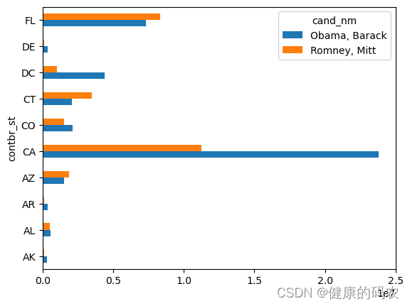
5. 按州进行统计

根据候选人和州对数据进行聚合，并绘制柱状图和饼图

grouped = fec_mrbo.groupby(["cand_nm", "contbr_st"])
totals = grouped["contb_receipt_amt"].sum().unstack(level=0).fillna(0)
totals = totals[totals.sum(axis="columns") > 100000]
totals.head(10)

cand_nm	Obama, Barack	Romney, Mitt
contbr_st
AK	281840.15	86204.24
AL	543123.48	527303.51
AR	359247.28	105556.00
AZ	1506476.98	1888436.23
CA	23824984.24	11237636.60
CO	2132429.49	1506714.12
CT	2068291.26	3499475.45
DC	4373538.80	1025137.50
DE	336669.14	82712.00
FL	7318178.58	8338458.81

绘制水平条形图

totals[:10].plot(kind='barh')

<Axes: ylabel='contbr_st'>

在这里插入图片描述

绘制饼图

totals[:5].plot(kind='pie', subplots=True, legend=False, autopct='%.2f')

array([<Axes: ylabel='Obama, Barack'>, <Axes: ylabel='Romney, Mitt'>],
      dtype=object)

在这里插入图片描述

对各行除以总赞助额，就会得到各候选人在各州的总赞助额比例

percent = totals.div(totals.sum(axis="columns"), axis="index")
percent.head(10)

cand_nm	Obama, Barack	Romney, Mitt
contbr_st
AK	0.765778	0.234222
AL	0.507390	0.492610
AR	0.772902	0.227098
AZ	0.443745	0.556255
CA	0.679498	0.320502
CO	0.585970	0.414030
CT	0.371476	0.628524
DC	0.810113	0.189887
DE	0.802776	0.197224
FL	0.467417	0.532583

percent = totals.div(totals.sum(axis="columns"), axis="index")
percent.head(10)

cand_nm	Obama, Barack	Romney, Mitt
contbr_st
AK	0.765778	0.234222
AL	0.507390	0.492610
AR	0.772902	0.227098
AZ	0.443745	0.556255
CA	0.679498	0.320502
CO	0.585970	0.414030
CT	0.371476	0.628524
DC	0.810113	0.189887
DE	0.802776	0.197224
FL	0.467417	0.532583