第三章一些算法的代码实现

王大队长

已于 2022-07-09 10:16:02 修改

阅读量2.6k

点赞数 1

分类专栏：数字图像处理（冈萨雷斯）算法代码实现文章标签：图像处理

于 2022-04-12 22:59:06 首次发布

本文链接：https://blog.csdn.net/qq_55621259/article/details/124136550

版权

数字图像处理（冈萨雷斯）算法代码实现专栏收录该内容

6 篇文章 20 订阅

订阅专栏

灰度变换

（1）线性变换

图像的灰度集中在较亮的区域而导致图像偏亮，这个时候可以对图像的每一个像素灰度作线性拉伸。

原图像f(i,j)的灰度范围为[a,b]，线性变换后图像g(i,j)的范围为[a1,b1]

关系式为： $g(i,j) = a1+\frac{b1-a1}{b-a}[f(i,j)-a]$

MATLAB代码：

clc;clear all;
img=imread('dog.jfif');
img_gray=rgb2gray(img);
a1=50;b1=250;a=0;b=255;
figure(1)
subplot(2,2,1);imhist(img_gray);
subplot(2,2,2);imshow(img_gray);
img_gray_tran = a1+(b1-a1)/(b-a)*(img_gray-a);
subplot(2,2,3);imhist(img_gray_tran);
subplot(2,2,4);imshow(img_gray_tran);

结果：

可见将灰度值从本身的0~255变换到50~250后的变换

（2）图像反转

s=L-1-r，s为变换后的灰度，r为原式灰度，原式灰度级范围记为[0,L-1]

MATLAB代码

clc;clear all;
img=imread('dog.jfif');
img_gray=rgb2gray(img);
img_gray_tran =255-img_gray;
figure(1)
subplot(2,2,1);imhist(img_gray);
subplot(2,2,2);imshow(img_gray);
subplot(2,2,3);imhist(img_gray_tran);
subplot(2,2,4);imshow(img_gray_tran);

（3）对数变换

s=c*log(1+r)

MATLAB代码

clc;clear all;
img=imread('dog.jfif');
img_gray=im2double(rgb2gray(img));
img_gray_tran =log(img_gray+1);
figure(1)
subplot(2,2,1);imhist(img_gray);
subplot(2,2,2);imshow(img_gray);
subplot(2,2,3);imhist(img_gray_tran);
subplot(2,2,4);imshow(img_gray_tran);

注意：第三行加im2double是为了防止溢出(uint8最大值是255,255再加1后就溢出了)

PYTHON代码(多熟悉下matplotlib)：

import cv2#cv2是BGR而不是RGB
import numpy as np #这个库用于随机生成和矩阵运算
import matplotlib.pyplot as plt
img = cv2.imread('dog.jfif')#用这个函数代替cv2.imread函数能使用含中文的文件名
image = cv2.cvtColor(img, cv2.COLOR_BGR2GRAY)
def log(img):
    output = np.log(1.0 + img)
    output = np.uint8(output + 0.5)
    return output
output=log(img)
plt.subplot(2,1,1)
plt.imshow(img,cmap = 'gray', interpolation = 'bicubic')
plt.title('original pictrue')
plt.xticks([]), plt.yticks([])#隐藏x轴和y轴刻度

plt.subplot(2,1,2)
plt.imshow(42*output,cmap = 'gray', interpolation = 'bicubic')#为什么乘42，因为不乘的话灰度值只有5左右，看起来全是黑的
plt.title('picture after log tran')
plt.xticks([]), plt.yticks([])
plt.show()

可见确实起到了对数变换的作用。注意！！！灰度化的图，在matplotlib里显示图像不是灰色的，这里因为通道转换问题，这里我们在OpenCV中显示则正常。

（4）分段线性变换

可以起到对比度拉伸和灰度级分层的作用。

PYTHON代码：

import cv2#cv2是BGR而不是RGB
img = cv2.imread('dog.jfif')#用这个函数代替cv2.imread函数能使用含中文的文件名
image = cv2.cvtColor(img, cv2.COLOR_BGR2GRAY)
def Pltrans(img):
    # r=np.copy(img)
    row,column=img.shape
    for i in range(row):
        for j in range(column):
            if img[i][j]<90:
                img[i][j]*=0.2
            if img[i][j]>90 and img[i][j]<160:
                img[i][j]*=3
            if img[i][j]>160:
                img[i][j]*=0.8
    return img
image1=Pltrans(image)
cv2.imshow("image1",image1)
cv2.waitKey(0)

运行结果：

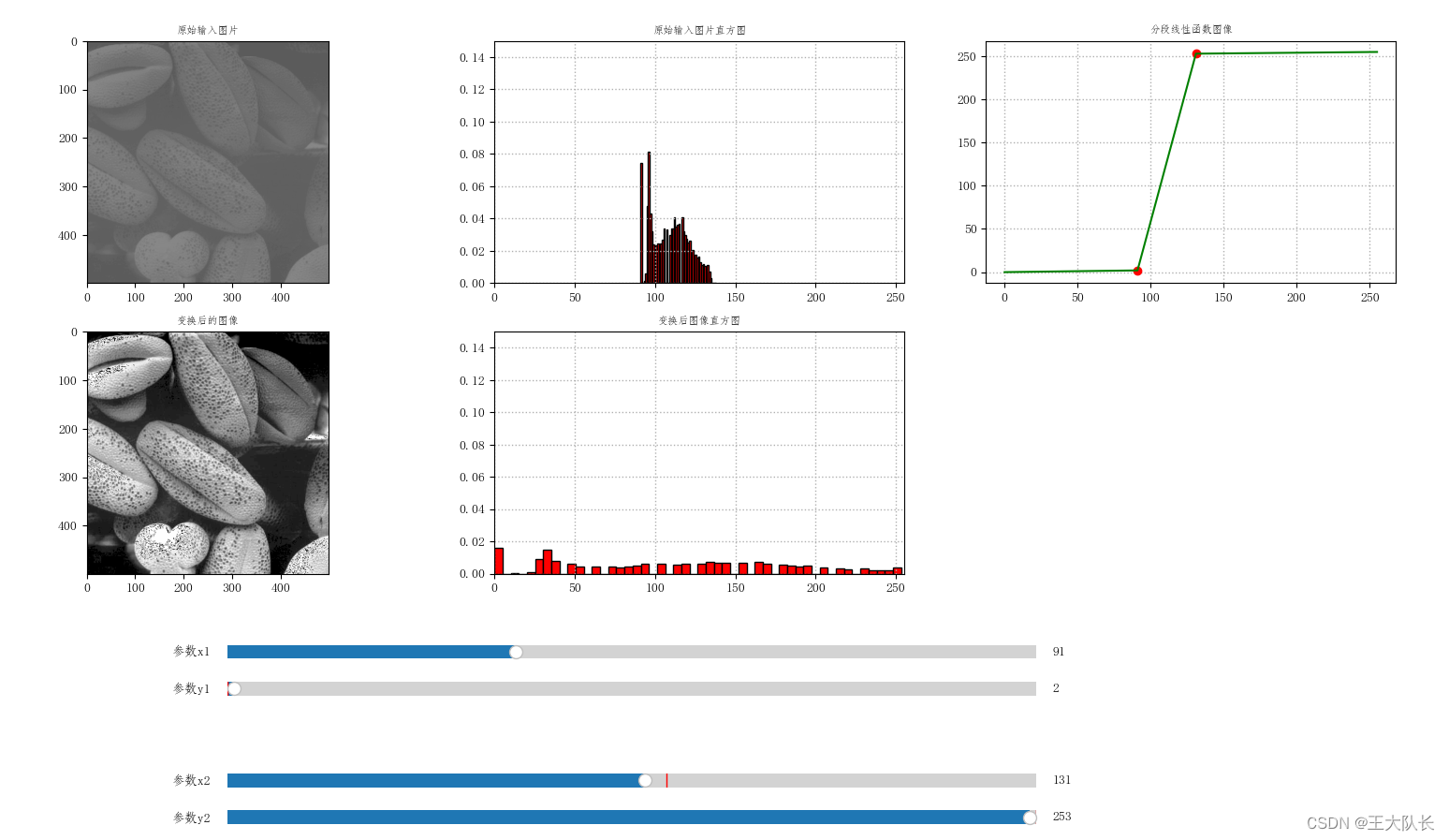
下面调用slider控件来实时更新我们的这个分段线性函数从而实时更新图像：

import cv2
import numpy as np
import matplotlib.pyplot as plt
from matplotlib.widgets import Slider #调用Slider滑块控件

def set_chinese(): #使得画图时的标题可以为中文
    import matplotlib
    print("[INFO] matplotlib版本为: %s" % matplotlib.__version__)
    matplotlib.rcParams['font.sans-serif'] = ['FangSong']
    matplotlib.rcParams['axes.unicode_minus'] = False

def three_line_trans(x,x1,y1,x2,y2):
    if x1==0 or x1==x2 or x2==255:
        print("[INFO] x1={},x2{} ->调用此函数必须满足: x1≠x2且x2≠255以及x1≠0")
        return None

    #【快速算法】
    m1 = (x<x1)
    m2 = (x>x1)&(x<x2)
    m3 = (x>x2)
    output = (y1*x/x1)*m1 + (((y2-y1)/(x2-x1))*(x-x1)+y1)*m2 + (((255-y2)/(255-x2))*(x-x2)+y2)*m3

    # 3.获取分段线性函数的点集，用于绘制函数图像
    x_point = np.arange(0, 256, 1)
    cond2 = [True if (i >= x1 and i <= x2) else False for i in x_point] #!!!不能直接写x1<=x_point<=x2,否则报错。暂时不知道为什么不能双向
    y_point = (y1 / x1 * x_point) * (x_point < x1) \
              + ((y2 - y1) / (x2 - x1) * (x_point - x1) + y1) * (cond2) \
              + ((255 - y2) / (255 - x2) * (x_point - x2) + y2) * (x_point > x2)

    return output, x_point, y_point

def update_trans(val):
    # 读入4个滑动条的值
    x1, y1 = slider_x1.val, slider_y1.val
    x2, y2 = slider_x2.val, slider_y2.val
    if x1>=x2:
        x1 = x2-1
    if y1>=y2:
        y1 = y2-1
    output, x_point, y_point = three_line_trans(img_original1, x1=x1, y1=y1, x2=x2, y2=y2)
    ax3.clear()
    ax3.set_title('分段线性函数图像', fontsize=8)
    ax3.grid(True, linestyle=':', linewidth=1)
    ax3.plot([x1, x2], [y1, y2], 'ro')
    ax3.plot(x_point, y_point, 'g')

    ax4.clear()
    ax4.set_title('变换后的图像', fontsize=8)
    ax4.imshow(output, cmap='gray', vmin=0, vmax=255)

    ax5.clear()
    ax5.set_title('变换后图像直方图', fontsize=8)
    ax5.hist(output.flatten(),bins=50, density=True, color='r', edgecolor='k')
    ax5.set_xlim(0, 255)  # 设置x轴分布范围
    ax5.set_ylim(0, 0.15)  # 设置y轴分布范围
    ax5.grid(True, linestyle=':', linewidth=1)


if __name__ == '__main__':
    set_chinese()
    img_original = cv2.imread(r'Fig0316(2)(2nd_from_top).tif')
    img_original1 = cv2.cvtColor(img_original, cv2.COLOR_BGR2GRAY)


    fig = plt.figure()
    ax1 = fig.add_subplot(231)
    ax2 = fig.add_subplot(232)
    ax3 = fig.add_subplot(233)
    ax4 = fig.add_subplot(234)
    ax5 = fig.add_subplot(235)

    ax1.set_title('原始输入图片',fontsize=8)
    ax1.imshow(img_original1,cmap='gray',vmin=0,vmax=255) #官方文档：https://matplotlib.org/stable/api/_as_gen/matplotlib.axes.Axes.imshow.html#matplotlib.axes.Axes.imshow
    ax2.set_title('原始输入图片直方图',fontsize=8)
    ax2.hist(img_original1.flatten(), bins=50, density=True, color='r', edgecolor='k') #bin属性控制直方图横条的数量, density为True则显示的是概率密度
    ax2.set_xlim(0, 255)  # 设置x轴分布范围
    ax2.set_ylim(0, 0.15)  # 设置y轴分布范围
    ax2.grid(True, linestyle=':', linewidth=1)

    plt.subplots_adjust(bottom=0.3)
    x1 = plt.axes([0.25, 0.2, 0.45, 0.03], facecolor='lightgoldenrodyellow') #控制横轴的left,bottom,width,height位置和大小
    slider_x1 = Slider(x1, '参数x1', 0.0, 255.,
                       valfmt='%.f', valinit=91, valstep=1) #slider的输入x必须是一个Axes
    slider_x1.on_changed(update_trans)

    y1 = plt.axes([0.25, 0.16, 0.45, 0.03],
                  facecolor='lightgoldenrodyellow')
    slider_y1 = Slider(y1, '参数y1', 0.0, 255.,
                       valfmt='%.f', valinit=0, valstep=1)
    slider_y1.on_changed(update_trans)

    x2 = plt.axes([0.25, 0.06, 0.45, 0.03],
                  facecolor='white')
    slider_x2 = Slider(x2, '参数x2', 0.0, 254.,
                       valfmt='%.f', valinit=138, valstep=1) #valinit表示slider的点的初始位置（即滑块的初始值）
    slider_x2.on_changed(update_trans)

    y2 = plt.axes([0.25, 0.02, 0.45, 0.03],
                  facecolor='white')
    slider_y2 = Slider(y2, '参数y2', 0.0, 255.,
                       valfmt='%.f', valinit=255, valstep=1)
    slider_y2.on_changed(update_trans)

    slider_x1.set_val(91)
    slider_y1.set_val(91)
    slider_x2.set_val(138)
    slider_y2.set_val(138)
    #plt.tight_layout()
    plt.show()

结果：（可以看到有个划钮，实际效果是可以拖动这个划钮的）

（5）直方图均衡化

import cv2#cv2是BGR而不是RGB
import numpy as np #这个库用于随机生成和矩阵运算
import matplotlib.pyplot as plt
img = cv2.imread('Fig0316(2)(2nd_from_top).tif')#用这个函数代替cv2.imread函数能使用含中文的文件名
image1 = cv2.cvtColor(img, cv2.COLOR_BGR2GRAY)
image2=cv2.equalizeHist(image1)#直方图均衡化函数
plt.subplot(2,2,1)
plt.hist(image1.ravel(), 256)
plt.rcParams["font.family"] = ["sans-serif"]
plt.rcParams["font.sans-serif"] = ['SimHei']
plt.title('直方图',fontproperties="SimHei")
plt.subplot(2,2,2)
plt.imshow(image1,cmap = 'gray',vmin=0, vmax=255)
plt.subplot(2,2,3)
plt.hist(image2.ravel(), 256)
plt.rcParams["font.family"] = ["sans-serif"]
plt.rcParams["font.sans-serif"] = ['SimHei']
plt.title('直方图均衡',fontproperties="SimHei")
plt.subplot(2,2,4)
plt.imshow(image2,cmap = 'gray')
plt.show()

上面的代码用了官方的直方图均衡化函数，下面给出自己写的直方图均衡化函数（只能显示均衡后的直方图，不对图片进行均衡。若想对图片进行均衡，自行将均衡后的元素存进一个二维数组中）

import numpy as np #这个库用于随机生成和矩阵运算
import matplotlib.pyplot as plt
import cv2#cv2是BGR而不是RGB
def origin_histogram(img): #将灰度值存储到一个数组中
    histogram=np.zeros(256,dtype = np.uint8)
    #img=np.array(img)
    for i in range(img.shape[0]):
        for j in range(img.shape[1]):
            k=img[i][j]
            histogram[k]=histogram[k]+1
    return histogram
def equalization_histogram(histogram,img): #将这个数组进行均衡化后存入新的数组中
    pr=np.zeros(256)
    for i in range(256):
        pr[i]=histogram[i]/(img.shape[0]*img.shape[1])

    temp=0
    sk=np.zeros(256)
    for i in range(len(pr)):
        temp+=pr[i]
        sk[i]=max(histogram)*temp
    histogram_equalization=np.round(sk)
    histogram_equalization=[int(x) for x in histogram_equalization]#对整个数组元素进行强制取整
    print(histogram_equalization)
    return histogram_equalization
if __name__=='__main__': #对数组进行画图得到直方图
    img = cv2.imread('Fig0316(2)(2nd_from_top).tif')  # 用这个函数代替cv2.imread函数能使用含中文的文件名
    img1=cv2.cvtColor(img,cv2.COLOR_BGR2GRAY)
    aaa=origin_histogram(img1)
    bbb=equalization_histogram(aaa,img1)
    x=np.arange(256)
    plt.subplot(1,2,1)
    plt.plot(x,aaa)
    plt.title('origin histogram')
    plt.subplot(1,2,2)
    plt.plot(x,bbb)
    plt.title('histogram after rqualization')
    plt.show()

运行结果：

推荐一篇写得很清晰的直方图均衡化原理文章：

(2条消息) 【图像处理算法】直方图均衡化_桂哥317的博客-CSDN博客_直方图均衡化

（6）均值滤波器、中值滤波器与高斯滤波器对椒盐噪声的影响：

#比较均值滤波与中值滤波对椒盐噪声的效果(这两个滤波器都是设置成正方形的size*size的)
import numpy as np
import matplotlib.pyplot as plt
import cv2
from math import exp
#均值滤波器
def Mean_filter(img,size):
    img_new=np.zeros((img.shape[0],img.shape[1]),dtype='uint8')

    for i in range(img.shape[0]):
        for j in range(img.shape[1]):
            sum, p = 0, 0
            for m in range(i-size//2,i+size-size//2):#为什么是size-size//2,因为range函数第二个参数减1才是真正的最后一个元素！
                for n in range(j-size//2,j+size-size//2):
                    if m<0 or m>=img.shape[0] or n<0 or n>=img.shape[1]:#这个语句：边缘处的中心像素少的就不加，不补零
                        continue
                    else:
                        sum+=img[m,n]
                        p+=1
            img_new[i,j]=sum/p
    return img_new
#取中位数函数
def get_median(array):
    a=0
    if len(array)%2==1:
        return array[int((len(array)-1)/2)]
    else:
        a=(array[int(len(array) / 2)] + array[int(len(array) / 2) - 1]) / 2
        return  a
#中值滤波器
def median_filter(img,size):
    img = np.array(img, dtype='int')#转换成int型防止像素加减溢出
    img_new = np.zeros((img.shape[0], img.shape[1]), dtype='uint8')
    for i in range(img.shape[0]):
        for j in range(img.shape[1]):
            array=[]
            for m in range(i-size//2,i+size-size//2):
                for n in range(j-size//2,j+size-size//2):
                    if m<0 or m>=img.shape[0] or n<0 or n>=img.shape[1]:
                        continue
                    else:
                        array.append(img[m,n])
            array=sorted(array)#把数组排序方便取中位数
            img_new[i,j]=int(get_median(array))
    img = np.array(img, dtype='uint8')#执行完像素加减后变回uint型
    return img_new
#高斯滤波器
def Gaussian_filter(img): #delta=3
    img = np.array(img, dtype='int')  # 转换成int型防止像素加减溢出
    img_new=np.copy(img)
    for i in range(1,img.shape[0]-1):#去掉边缘
        for j in range(1,img.shape[1]-1):
            img_new[i,j]=np.sum(Gaussian_operator*img[i-1:i+2,j-1:j+2])
    return img_new

if __name__=='__main__':
    Gaussian_operator=np.array([[exp(-1/9),exp(-1/18),exp(-1/9)],[exp(-1/18),exp(0),exp(-1/18)],[exp(-1/9),exp(-1/18),exp(-1/9)]])
    img=cv2.imread('Fig0335(a)(ckt_board_saltpep_prob_pt05).tif')#shape:440*455
    img1=cv2.cvtColor(img,cv2.COLOR_BGR2GRAY)
    img_new1=Mean_filter(img1,3)
    img_new2=median_filter(img1,3)
    img_new3=Gaussian_filter(img1)
    plt.subplot(2, 2, 1)
    plt.imshow(img1,cmap='gray')
    plt.title('original')
    plt.subplot(2, 2, 2)
    plt.imshow(img_new1, cmap='gray')
    plt.title('picture after Mean_filter')
    plt.subplot(2, 2, 3)
    plt.imshow(img_new2, cmap='gray')
    plt.title('picture after median_filter')
    plt.subplot(2,2,4)
    plt.imshow(img_new3, cmap='gray')
    plt.title('picture after Gaussian_filter')
    plt.show()

运行结果：

（7）使用拉普拉斯算子的图像锐化

在这里使用的是[[1,1,1],[1,-8,1],[1,1,1]]模板，可自行更改自己需要的模板

PYTHON代码（网上版本）：

#拉普拉斯算子
import cv2
import matplotlib.pyplot as plt
import numpy as np
def Laplace_filter(img): #拉普拉斯锐化操作
    img=np.array(img,dtype='int')
    img_new=np.copy(img)
    r,w=img.shape
    for i in range(1,r-1):
        for j in range(1,w-1):
            R=np.sum(Laplace_operator*img[i-1:i+2,j-1:j+2])
            img_new[i,j]=img[i,j]-R
    return img_new
if __name__=='__main__':
    Laplace_operator=np.array([[1,1,1],[1,-8,1],[1,1,1]]) #拉普拉斯模板
    img = cv2.imread('Fig0338(a)(blurry_moon).tif')  # shape:440*455
    img1 = cv2.cvtColor(img, cv2.COLOR_BGR2GRAY)
    img2 = Laplace_filter(img1)
    plt.subplot(1, 2, 1)
    plt.imshow(img1, cmap='gray')
    plt.title('original picture')
    plt.subplot(1, 2, 2)
    plt.imshow(img2, cmap='gray')  # 将新生成的二维数组生成图片用plt.imshow，cv2.imshow不行
    plt.title('picture after Laplace operator')
    plt.show()

运行结果：

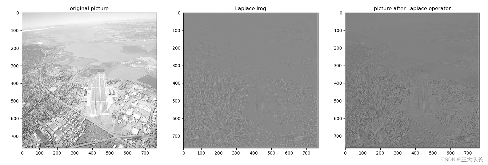
PYTHON代码（自己写的，含补零操作，且与教材上完全一致，先求出拉普拉斯图像，再用原图像加上拉普拉斯图像得到最终结果）

#拉普拉斯算子
import cv2
import matplotlib.pyplot as plt
import numpy as np
def Laplace_filter(img, kernel): #拉普拉斯锐化操作
    #img=np.array(img,dtype='int')
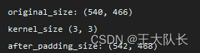
    print('original_size:', img.shape)
    print('kernel_size', kernel.shape)
    '''补零'''
    img = cv2.resize(img, (img.shape[1]+kernel.shape[1]-1, img.shape[0]+kernel.shape[0]-1)) #这里cv2.resize函数要反一下，详情
    img = np.array(img, dtype='int')
    img[0:kernel.shape[0]-1,:]=0
    img[:,0:kernel.shape[1] - 1] = 0
    img[img.shape[0]-kernel.shape[0]-2:,:] = 0
    img[:,img.shape[1] - kernel.shape[1] - 2:] = 0
    print('after_padding_size:',img.shape)

    R=np.copy(img) #用来接收拉普拉斯图像
    r,w=img.shape
    for i in range(1,r-1):
        for j in range(1,w-1):
            R[i,j]=np.sum(kernel*img[i-1:i+2,j-1:j+2])
    '''将拉普拉斯图像规定化到0~255'''
    min = np.min(R)
    max = np.max(R)
    R = R - min
    R = 255*(R/max)

    img = img - R #最终锐化结果
    return img, R
if __name__=='__main__':
    Laplace_operator=np.array([[1,1,1],[1,-8,1],[1,1,1]]) #拉普拉斯模板
    img = cv2.imread('Fig0338(a)(blurry_moon).tif')  # shape:440*455
    img1 = cv2.cvtColor(img, cv2.COLOR_BGR2GRAY)
    img2, R = Laplace_filter(img1, Laplace_operator)
    plt.subplot(1, 3, 1)
    plt.imshow(img1, cmap='gray')
    plt.title('original picture')
    plt.subplot(1, 3, 2)
    plt.imshow(R, cmap='gray')  # 将新生成的二维数组生成图片用plt.imshow，cv2.imshow不行
    plt.title('Laplace img')
    plt.subplot(1, 3, 3)
    plt.imshow(img2, cmap='gray')  # 将新生成的二维数组生成图片用plt.imshow，cv2.imshow不行
    plt.title('picture after Laplace operator')
    plt.show()

结果：

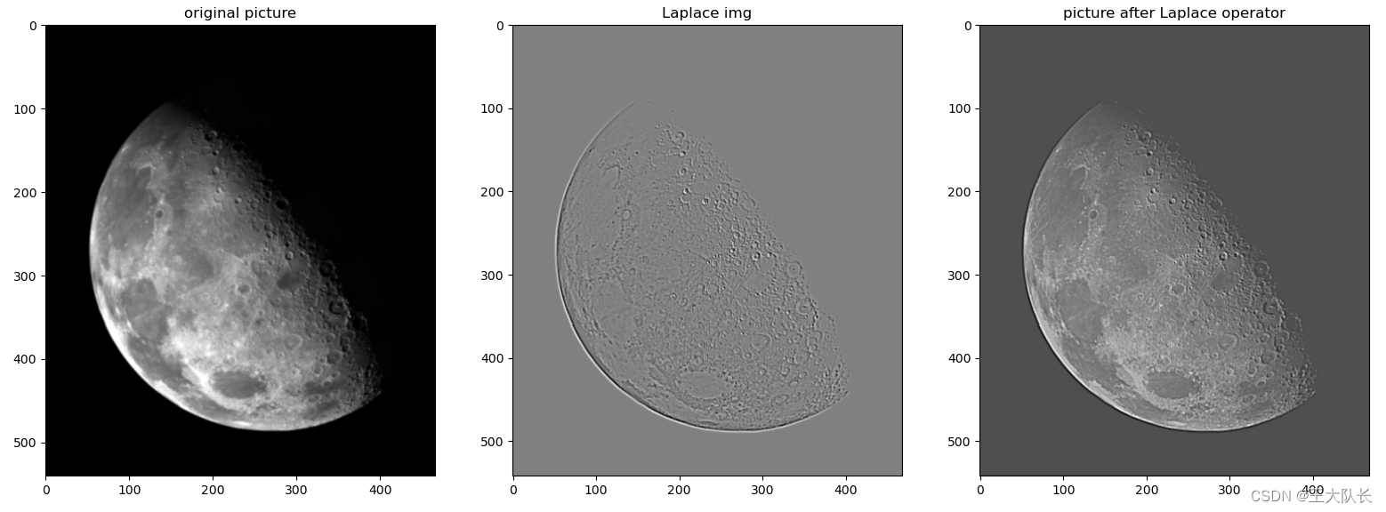
换张图片试试效果：

(8)使用Soble算子的的梯度进行边缘增强

PYTHON代码：

import cv2
import matplotlib.pyplot as plt
import numpy as np

#Soble算子
def Sobel(img):
    img = np.array(img, dtype='int')
    img_new = np.copy(img)
    r, w = img.shape
    for i in range(1, r - 1):
        for j in range(1, w - 1):
            img_new[i,j] = abs(np.sum(Sobel_operator1 * img[i - 1:i + 2, j - 1:j + 2]))+abs(np.sum(Sobel_operator2 * img[i - 1:i + 2, j - 1:j + 2]))
    return img_new
if __name__=='__main__':
    Sobel_operator1=np.array([[-1,-2,-1],[0,0,0],[1,2,1]])
    Sobel_operator2=np.array([[-1,0,1],[-2,0,2],[-1,0,1]])
    img=cv2.imread('Fig0342(a)(contact_lens_original).tif')
    img1 = cv2.cvtColor(img, cv2.COLOR_BGR2GRAY)
    img3=Sobel(img1)
    plt.subplot(1,2,1)
    plt.imshow(img1,cmap='gray')
    plt.title('original picture')
    plt.subplot(1,2,2)
    plt.imshow(img3,cmap='gray')
    plt.title('picture after Sobel')
    plt.show()

运行结果：

未完待续...

王大队长

关注

1
点赞
踩
4

收藏

觉得还不错? 一键收藏
0
评论
第三章一些算法的代码实现

灰度变换（1）线性变换图像的灰度集中在较亮的区域而导致图像偏亮，这个时候可以对图像的每一个像素灰度作线性拉伸。原图像f(i,j)的灰度范围为[a,b]，线性变换后图像g(i,j)的范围为[a1,b1]关系式为：MATLAB代码：clc;clear all;img=imread('dog.jfif');img_gray=rgb2gray(img);a1=50;b1=250;a=0;b=255;figure(1)subplot(2,2,1);imhist(img_gray).
复制链接

扫一扫