softmax回归

一、概念

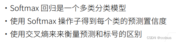
1、softmax回归其实是一个分类问题

2、回归估计一个连续值，单连续数值输出，跟真实值的区别作为损失。

3、多类分类

（1）分类预测一个离散类别，多个输出，输出为第i类的置信度

（2）均方损失

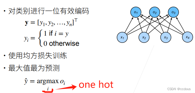
独热编码：将类别变量转换为二进制矩阵的编码方式，常用于机器学习和深度学习中处理分类数据。其基本思想是将每个类别表示为一个向量，其中只有一个位置的值为1，其余位置的值为0。

（3）无校验比例

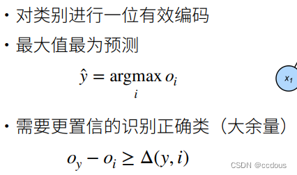
使对正确类别的置信特别大，将正确类与非正确类大大拉开距离使其差距大于某一阈值

（4）校验比例

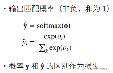
对向量处理使其成为概率（全为非负，总和为1）

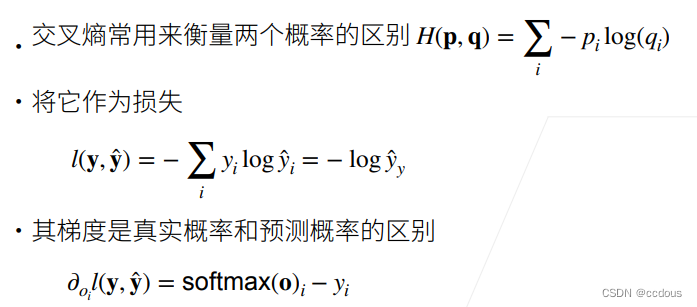
4、交叉熵损失

5、总结

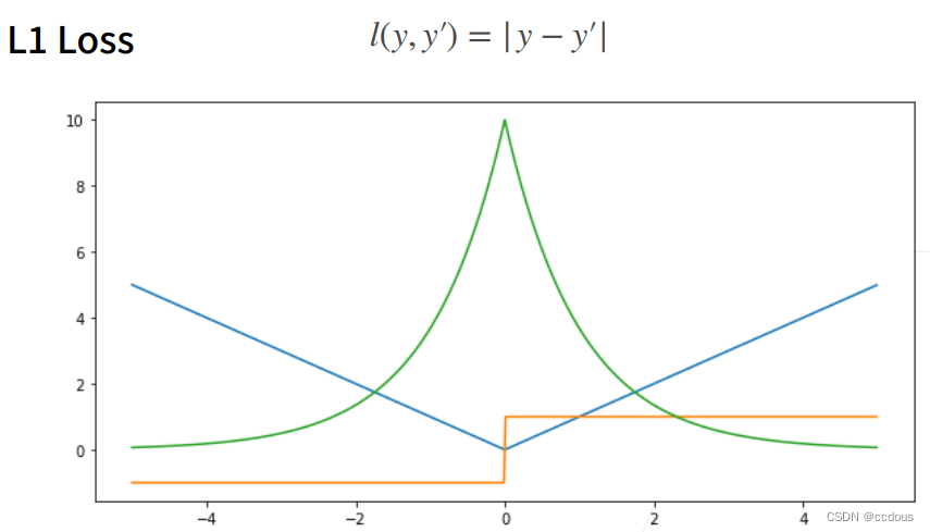
二、损失函数：衡量预测值和真实值之间的区别

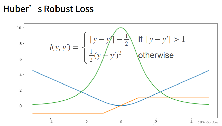
1、蓝色：y=0时，变化预测值y’的函数；绿色：似然函数e^(-l())，是高斯分布；黄色：梯度函数

2、导数决定如何更新梯度

3、L2 Loss

损失函数的导函数是一条直线，说明损失函数越靠近原点变化越小，所以梯度更新就越慢

4、L1 Loss

5、Huber's Robust Loss：将L1与L2进行优化

三、图像分类数据集

    MNIST数据集是图像分类中广泛使用的数据集之一，但作为基准数据集过于简单。 我们将使用类似但更复杂的Fashion-MNIST数据集 。

1、导包

%matplotlib inline
import torch
import torchvision
from torch.utils import data
from torchvision import transforms
from d2l import torch as d2l

2、读取数据集

（1）数据集下载

# 通过ToTensor实例将图像数据从PIL类型变换成32位浮点数格式，
# 并除以255使得所有像素的数值均在0～1之间
trans = transforms.ToTensor()
mnist_train = torchvision.datasets.FashionMNIST(
    #train=True表示训练数据集
    root="../data", train=True, transform=trans, download=True)
mnist_test = torchvision.datasets.FashionMNIST(
    #train=False表示测试数据集
    root="../data", train=False, transform=trans, download=True)

（2）数字标签索引及其文本名称之间进行转换

def get_fashion_mnist_labels(labels):  #@save
    """返回Fashion-MNIST数据集的文本标签"""
    text_labels = ['t-shirt', 'trouser', 'pullover', 'dress', 'coat',
                   'sandal', 'shirt', 'sneaker', 'bag', 'ankle boot']
    return [text_labels[int(i)] for i in labels]

（3）可视化样本函数：这个我不了解啊，老师就说同学们看看，呜呜呜呜

def show_images(imgs, num_rows, num_cols, titles=None, scale=1.5):  #@save
    """绘制图像列表"""
    figsize = (num_cols * scale, num_rows * scale)
    _, axes = d2l.plt.subplots(num_rows, num_cols, figsize=figsize)
    axes = axes.flatten()
    for i, (ax, img) in enumerate(zip(axes, imgs)):
        if torch.is_tensor(img):
            # 图片张量
            ax.imshow(img.numpy())
        else:
            # PIL图片
            ax.imshow(img)
        ax.axes.get_xaxis().set_visible(False)
        ax.axes.get_yaxis().set_visible(False)
        if titles:
            ax.set_title(titles[i])
    return axes

3、读取小批量

batch_size = 256
def get_dataloader_workers():  #@save
    """使用4个进程来读取数据"""
    return 4

train_iter = data.DataLoader(mnist_train, batch_size, shuffle=True,
                             num_workers=get_dataloader_workers())

4、整合组件（就是总和）

#例子里的图片是(1,28,28),如果我们后面要用到大的图片，可以使用resize去更改大小
def load_data_fashion_mnist(batch_size, resize=None):  #@save
    """下载Fashion-MNIST数据集，然后将其加载到内存中"""
    trans = [transforms.ToTensor()]
    if resize:
        trans.insert(0, transforms.Resize(resize))
    trans = transforms.Compose(trans)
    mnist_train = torchvision.datasets.FashionMNIST(
        root="../data", train=True, transform=trans, download=True)
    mnist_test = torchvision.datasets.FashionMNIST(
        root="../data", train=False, transform=trans, download=True)
    return (data.DataLoader(mnist_train, batch_size, shuffle=True,
                            num_workers=get_dataloader_workers()),
            data.DataLoader(mnist_test, batch_size, shuffle=False,
                            num_workers=get_dataloader_workers()))

四、softmax回归的从零开始实现

1、导包

import torch
from IPython import display
from d2l import torch as d2l

batch_size = 256
train_iter, test_iter = d2l.load_data_fashion_mnist(batch_size)

2、初始化模型参数

num_inputs = 784
num_outputs = 10

W = torch.normal(0, 0.01, size=(num_inputs, num_outputs), requires_grad=True)
b = torch.zeros(num_outputs, requires_grad=True)

3、定义softmax操作

def softmax(X):
    #对于任何随机输入，我们将每个元素变成一个非负数
    X_exp = torch.exp(X)
    partition = X_exp.sum(1, keepdim=True)
    return X_exp / partition  # 这里应用了广播机制

4、定义模型

def net(X):
    #这里W.shape[0]=784，X是256*28*28，X.reshape((-1, W.shape[0]))令X成为256*784的矩阵
    #X*W+b的值
    return softmax(torch.matmul(X.reshape((-1, W.shape[0])), W) + b)

5、定义损失函数

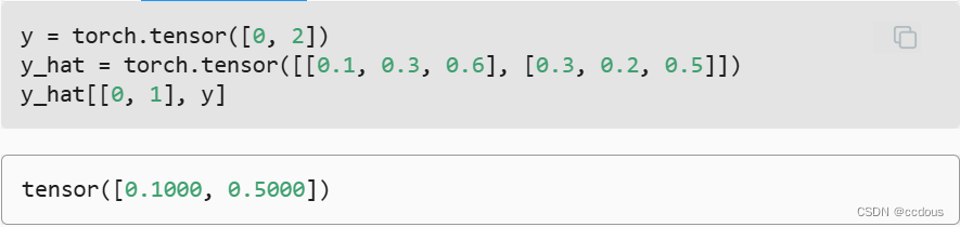
#y是真实标号，y_hat是按类别分来的预测概率
def cross_entropy(y_hat, y):
    #y_hat[]指取出其中指定位置元素的列表，放一个例子在下面
    #y_hat[range(len(y_hat)), y]取出了真实标号的预测概率
    #-logy为计算交叉熵损失
    return -torch.log(y_hat[range(len(y_hat)), y])

cross_entropy(y_hat, y)

6、分类精度

def accuracy(y_hat, y):  #@save
    """计算预测正确的数量"""
    if len(y_hat.shape) > 1 and y_hat.shape[1] > 1:
        #我们取出预测的每一类别的最大估计值的下标
        y_hat = y_hat.argmax(axis=1)
    #将估计下标与真实下标做比较拿到一个关于预测值的bool类型的tensor
    cmp = y_hat.type(y.dtype) == y
    #将cmptensor转化为数值类型求和
    return float(cmp.type(y.dtype).sum())

#取平均，得到精度率
accuracy(y_hat,y)/len(y)

（2）任意数据迭代器data_iter可访问的数据集， 我们可以评估在任意模型net的精度

def evaluate_accuracy(net, data_iter):  #@save
    """计算在指定数据集上模型的精度"""
    if isinstance(net, torch.nn.Module):
        net.eval()  # 将模型设置为评估模式
    metric = Accumulator(2)  # 正确预测数、预测总数
    with torch.no_grad():
        for X, y in data_iter:
            #accuracy(net(X), y 评估值与真实值预测精度
            metric.add(accuracy(net(X), y), y.numel())
    #分类正确的样本数和总样本数的比例
    return metric[0] / metric[1]

实用程序类Accumulator，用于对多个变量进行累加

class Accumulator:  #@save
    """在n个变量上累加"""
    def __init__(self, n):
        self.data = [0.0] * n

    def add(self, *args):
        self.data = [a + float(b) for a, b in zip(self.data, args)]

    def reset(self):
        self.data = [0.0] * len(self.data)

    def __getitem__(self, idx):
        return self.data[idx]

7、训练

（1）训练模型一个迭代周期

def train_epoch_ch3(net, train_iter, loss, updater):  #@save
    """训练模型一个迭代周期（定义见第3章）"""
    # 将模型设置为训练模式
    if isinstance(net, torch.nn.Module):
        net.train()
    # 训练损失总和、训练准确度总和、样本数
    metric = Accumulator(3)
    for X, y in train_iter:
        # 计算梯度并更新参数
        y_hat = net(X)
        l = loss(y_hat, y)
        if isinstance(updater, torch.optim.Optimizer):
            # 使用PyTorch内置的优化器和损失函数
            updater.zero_grad()
            l.mean().backward()
            updater.step()
        else:
            # 使用定制的优化器和损失函数
            l.sum().backward()
            updater(X.shape[0])
        metric.add(float(l.sum()), accuracy(y_hat, y), y.numel())
    # 返回训练损失和训练精度
    return metric[0] / metric[2], metric[1] / metric[2]

（2）训练函数

def train_ch3(net, train_iter, test_iter, loss, num_epochs, updater):  #@save
    """训练模型（定义见第3章）"""
    #可视化
    animator = Animator(xlabel='epoch', xlim=[1, num_epochs], ylim=[0.3, 0.9],
                        legend=['train loss', 'train acc', 'test acc'])
    #num_epochs轮循环
    for epoch in range(num_epochs):
        #训练模型、更新、拿回训练损失和训练精度
        train_metrics = train_epoch_ch3(net, train_iter, loss, updater)
        #在测试数据集上测试精度
        test_acc = evaluate_accuracy(net, test_iter)
        animator.add(epoch + 1, train_metrics + (test_acc,))
    train_loss, train_acc = train_metrics
    assert train_loss < 0.5, train_loss
    assert train_acc <= 1 and train_acc > 0.7, train_acc
    assert test_acc <= 1 and test_acc > 0.7, test_acc

（3）小批量随机梯度下降来优化模型的损失函数，设置学习率为0.1

lr = 0.1

def updater(batch_size):
    return d2l.sgd([W, b], lr, batch_size)

（4）使用

num_epochs = 10
d2l.train_ch3(net, train_iter, test_iter, loss, num_epochs, trainer)

五、简洁实现

1、导包

import torch
from torch import nn
from d2l import torch as d2l

batch_size = 256
train_iter, test_iter = d2l.load_data_fashion_mnist(batch_size)

2、初始化模型参数

# PyTorch不会隐式地调整输入的形状。因此，
# 我们在线性层前定义了展平层（flatten），来调整网络输入的形状
#第0维度保留，其余维度全部平展为向量，变成2维
net = nn.Sequential(nn.Flatten(), nn.Linear(784, 10))

def init_weights(m):
    if type(m) == nn.Linear:
        #初始化权重
        nn.init.normal_(m.weight, std=0.01)

net.apply(init_weights);

3、损失函数

loss = nn.CrossEntropyLoss(reduction='none')

4、优化算法（学习率为0.1的小批量随机梯度下降作为优化算法）

trainer = torch.optim.SGD(net.parameters(), lr=0.1)

5、训练

num_epochs = 10
d2l.train_ch3(net, train_iter, test_iter, loss, num_epochs, trainer)