分别利用线性回归、多项式回归分析工资与年限的关系

一、线性回归：

实验思路：

先分析线性回归的代码，然后结合Salary_dataset.csv内容分析，编写代码。

Salary_dataset.csv文件内容如下：

,YearsExperience,Salary
0,1.2000000000000002,39344.0
1,1.4000000000000001,46206.0
2,1.6,37732.0
3,2.1,43526.0
4,2.3000000000000003,39892.0
5,3.0,56643.0
6,3.1,60151.0
7,3.3000000000000003,54446.0
8,3.3000000000000003,64446.0
9,3.8000000000000003,57190.0
10,4.0,63219.0
11,4.1,55795.0
12,4.1,56958.0
13,4.199999999999999,57082.0
14,4.6,61112.0
15,5.0,67939.0
16,5.199999999999999,66030.0
17,5.3999999999999995,83089.0
18,6.0,81364.0
19,6.1,93941.0
20,6.8999999999999995,91739.0
21,7.199999999999999,98274.0
22,8.0,101303.0
23,8.299999999999999,113813.0
24,8.799999999999999,109432.0
25,9.1,105583.0
26,9.6,116970.0
27,9.7,112636.0
28,10.4,122392.0
29,10.6,121873.0

实验代码：

import pandas as pd
import numpy as np
from sklearn.linear_model import LinearRegression
from sklearn.metrics import mean_squared_error, r2_score
import matplotlib.pyplot as plt

# 1. 读取数据
data = pd.read_csv('Salary_dataset.csv')

# 假设数据是干净的，没有缺失值或异常值
X = data['YearsExperience'].values.reshape(-1, 1)  # 特征列
y = data['Salary'].values  # 目标变量列

# 2. 选取五个数据点作为训练集
# 这里我们随机选取五个数据点，你可以根据需要更改选取数据点的方式
train_indices = np.random.choice(len(data), 5, replace=False)
X_train = X[train_indices]
y_train = y[train_indices]

# 剩余的数据作为测试集
X_test = np.delete(X, train_indices, axis=0)
y_test = np.delete(y, train_indices, axis=0)

# 3. 训练线性回归模型
model = LinearRegression()
model.fit(X_train, y_train)

# 4. 评估模型
y_pred = model.predict(X_test)
mse = mean_squared_error(y_test, y_pred)
rmse = np.sqrt(mse)
r2 = r2_score(y_test, y_pred)

print(f'Mean Squared Error: {mse}')
print(f'Root Mean Squared Error: {rmse}')
print(f'R² score: {r2}')

# 5. 可视化结果
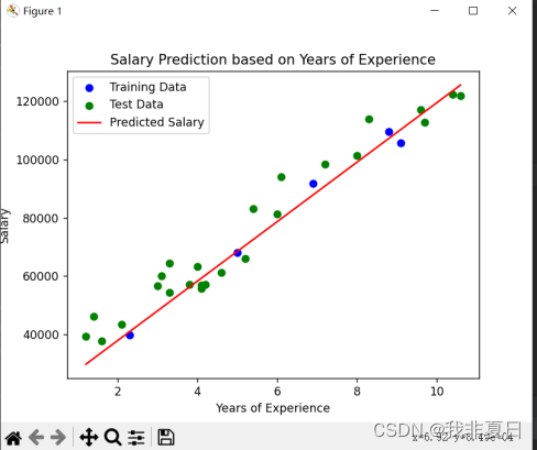
plt.scatter(X_train, y_train, color='blue', label='Training Data')
plt.scatter(X_test, y_test, color='green', label='Test Data')
plt.plot(X_test, y_pred, color='red', label='Predicted Salary')
plt.xlabel('Years of Experience')
plt.ylabel('Salary')
plt.title('Salary Prediction based on Years of Experience')
plt.legend()
plt.show()

实验结果：

二、多项式回归：

实验思路：

先分析多项式回归的代码，然后结合Salary_dataset.csv内容分析，编写代码。

实验代码：

import numpy as np
import pandas as pd
import matplotlib.pyplot as plt
from sklearn.pipeline import Pipeline
from sklearn.preprocessing import PolynomialFeatures
from sklearn.linear_model import LinearRegression

# 读取CSV文件
data = pd.read_csv('Salary_dataset.csv')
X = data['YearsExperience'].values.reshape(-1, 1)  # 特征
y = data['Salary'].values  # 目标变量


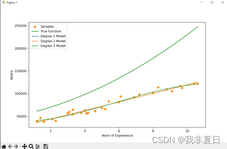
# 假设的真实函数（这里只是一个例子，实际上我们不知道真实函数）
def true_function(x):
    return 50000 + 8000 * x + 1000 * x ** 2  # 假设的真实工资与年限关系


# 创建X值的范围用于绘制真实函数和模型预测
X_plot = np.linspace(X.min(), X.max(), 100).reshape(-1, 1)
y_true = true_function(X_plot)

# 定义多项式次数
degrees = [1, 2, 3]

# 初始化图表和子图
plt.figure(figsize=(10, 6))
plt.scatter(X, y, color='darkorange', label='Samples')  # 绘制样本点
plt.plot(X_plot, y_true, color='green', label='True function')  # 绘制真实函数
plt.xlabel('Years of Experience')
plt.ylabel('Salary')
plt.legend(loc='upper left')

# 对每个多项式次数进行训练和可视化
for i, degree in enumerate(degrees):
    polynomial_features = PolynomialFeatures(degree=degree, include_bias=False)
    linear_regression = LinearRegression()
    pipeline = Pipeline([("polynomial_features", polynomial_features),
                         ("linear_regression", linear_regression)])
    pipeline.fit(X, y)

    # 使用管道进行预测
    y_plot = pipeline.predict(X_plot)

    # 绘制模型拟合曲线
    plt.plot(X_plot, y_plot, label=f'Degree {degree} Model')

# 显示图例
plt.legend(loc='best')
plt.show()

实验结果：