


特征工程
以下代码根据Abhishek Thakur在kaggle上的机器学习30天 (b站) (kaggle)可惜的是,我没有找到源代码,如果需要代码可以从其他人上传的代码里“盗取”。
我们首先导入需要的库函数
import numpy as np
import pandas as pd
from sklearn import preprocessing
from sklearn.model_selection import train_test_split
from sklearn.ensemble import RandomForestRegressor
from xgboost import XGBRegressor
from sklearn.metrics import mean_squared_error
数据如下,可以发现有数值型变量和分类型变量,下面我们对其进行操作

数值型变量
standardization
减去平均值,除以标准差(standardScaler)
    scaler = preprocessing.StandardScaler()
    xtrain[numerical_cols] = scaler.fit_transform(xtrain[numerical_cols])
    xvalid[numerical_cols] = scaler.transform(xvalid[numerical_cols])
    xtest[numerical_cols] = scaler.transform(xtest[numerical_cols])
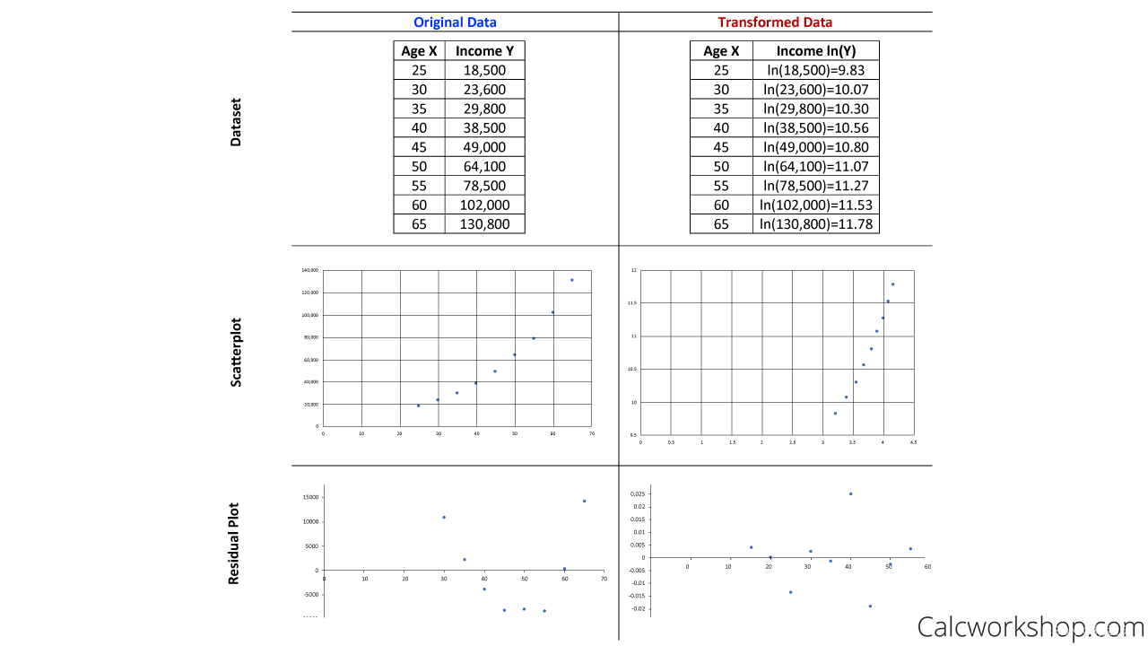
log_transformation(使其符合正态分布)
It’s one of several methods that you can use to transform datasets to achieve linearity .
This means it can help you obtain further insights into your data that may not be obvious at first.For example, notice how the original data below shows a nonlinear relationship. Well, after applying an exponential transformation, which takes the natural log of the response variable, our data becomes a linear function as seen in the side-by-side comparison of both scatterplots and residual plots.
“残差图”以回归方程的自变量为横坐标,以残差为纵坐标,将每一个自变量的残差描在该平面坐标上所形成的图形。当描绘的点围绕残差等于O的直线上下随机散布,说明回归直线对原观测值的拟合情况良好。否则,说明回归直线对原观测值的拟合不理想.。从“残差图”可以直观地看出残差的绝对数值都比较小,所描绘的点都在以O为横轴的直线上下随机散布,回归直线对各个观测值的拟合情况是良好的。说明变量X与y之间有显著的线性相关关系。
log1p就是
for col in numerical_cols:
    df[col] = np.log1p(df[col])
    df_test[col] = np.log1p(df_test[col])
polynomial features
如果有(a,b)两个特征,使用degree=2的二次多项式,则为(1,a, a^2, ab, b ,b^2)。以此类推。interaction_only就是只留下交互项,去掉1,a,b。
poly = preprocessing.PolynomialFeatures(degree=3, interaction_only=True, include_bias=False)
train_poly = poly.fit_transform(df[numerical_cols])
test_poly = poly.fit_transform(df_test[numerical_cols])
分类型变量
orinigalencoder
直接原始分类,a是1,b是2
 ordinal_encoder = preprocessing.OrdinalEncoder()
 xtrain[object_cols] = ordinal_encoder.fit_transform(xtrain[object_cols])
 xvalid[object_cols] = ordinal_encoder.fit_transform(xvalid[object_cols])
 #应该为transform
 xtest[object_cols] = ordinal_encoder.fit_transform(xtest[object_cols])
 #应该为transform
这里我写的时候突然发现一个问题,如果都对其使用fit_transform可能最后诞生的分类是不同的,如果单一fit后是能保证一一对应的。
你想对单个serie进行操作,就用label encoder.
onehot encoder
独热编码
    ohe = preprocessing.OneHotEncoder(sparse=False, handle_unknown="ignore")
    xtrain_ohe = ohe.fit_transform(xtrain[object_cols])
    xvalid_ohe = ohe.transform(xvalid[object_cols])
    xtest_ohe = ohe.transform(xtest[object_cols])
分类创造下的数值
df.groupbu(col)[col].transform()#不改变形状
df.groupbu(col)[col].agg()


 1万+
1万+


 被折叠的 条评论
为什么被折叠?
被折叠的 条评论
为什么被折叠?
 到【灌水乐园】发言


