从零开始实现类GPT模型

非黑非白Ress

已于 2024-08-15 01:59:39 修改

阅读量1k

点赞数 26

分类专栏：从零开始实现大语言模型文章标签： gpt pytorch

于 2024-08-15 01:37:00 首次发布

本文链接：https://blog.csdn.net/qq_63894862/article/details/141203649

版权

从零开始实现大语言模型专栏收录该内容

2 篇文章

订阅专栏

从零开始实现类GPT模型

前置

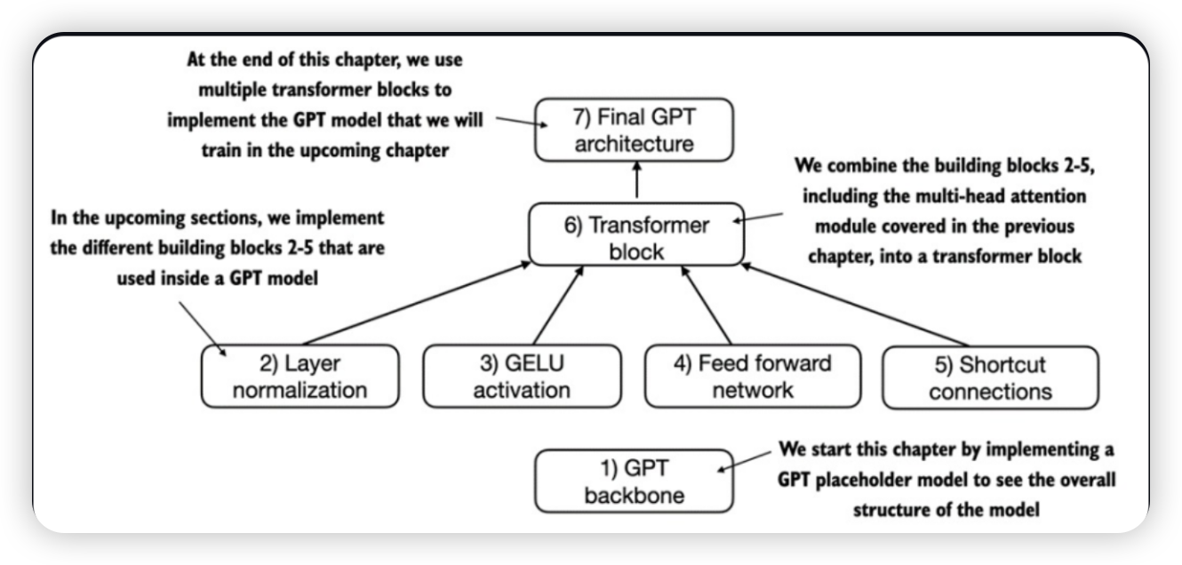
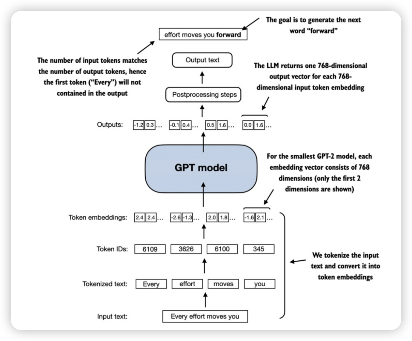
本文将从以下七个步骤，构建一个类GPT模型

配置参数

GPT - 2 的开源参数：

GPT_CONFIG_124M = {
	"vocab_size": 50257,      # 50257个单词的词汇表
    "context_length": 1024,   # 最大输入向量数
    "emb_dim": 768,           # 嵌入维度
    "n_heads": 12,            # 注意力头数
    "n_layers": 12,           # transformer数量
    "drop_rate": 0.1,         # 丢弃率10%
    "qkv_bias": False         # 偏向量
}

Token embeddings

import tiktoken
import torch

tokenizer = tiktoken.get_encoding("gpt2")
batch = []
txt1 = "Every effort moves you"
txt2 = "Every day holds a"

batch.append(torch.tensor(tokenizer.encode(txt1)))
batch.append(torch.tensor(tokenizer.encode(txt2)))
batch = torch.stack(batch, dim=0)
print(batch)

tensor([[6109, 3626, 6100,  345],
        [6109, 1110, 6622,  257]])

GPT backbone

DummyGPTModel：

import torch
import torch.nn as nn
class DummyGPTModel(nn.Module):
    def __init__(self, cfg):
        super().__init__()
        # 标记和位置嵌入
        self.tok_emb = nn.Embedding(cfg["vocab_size"], cfg["emb_dim"])
        self.pos_emb = nn.Embedding(cfg["context_length"], cfg["emb_dim"])
        # Dropout
        self.drop_emb = nn.Dropout(cfg["drop_rate"])
        # Transformer 模块
        self.trf_blocks = nn.Sequential(
            *[DummyTransformerBlock(cfg) for _ in range(cfg["n_layers"])])
        # 最终归一化
        self.final_norm = DummyLayerNorm(cfg["emb_dim"])
        # 线性输出层
        self.out_head = nn.Linear(
            cfg["emb_dim"], cfg["vocab_size"], bias=False)
    # 数据流
    def forward(self, in_idx):
        batch_size, seq_len = in_idx.shape
        tok_embeds = self.tok_emb(in_idx)
        pos_embeds = self.pos_emb(torch.arange(seq_len, device=in_idx.device))
        x = tok_embeds + pos_embeds
        x = self.drop_emb(x)
        x = self.trf_blocks(x)
        x = self.final_norm(x)
        logits = self.out_head(x)
        return logits    
 
 # Transformer 模块 
class DummyTransformerBlock(nn.Module):
    def __init__(self, cfg):
        super().__init__()
    def forward(self, x):
        return x

# 归一化 模块
class DummyLayerNorm(nn.Module):
    def __init__(self, normalized_shape, eps=1e-5):
        super().__init__()
    def forward(self, x):
        return x

测试


torch.manual_seed(123)
model = DummyGPTModel(GPT_CONFIG_124M)
logits = model(batch)
print("Output shape:", logits.shape)
print(logits)

Output shape: torch.Size([2, 4, 50257])
tensor([[[-0.9289,  0.2748, -0.7557,  ..., -1.6070,  0.2702, -0.5888],
         [-0.4476,  0.1726,  0.5354,  ..., -0.3932,  1.5285,  0.8557],
         [ 0.5680,  1.6053, -0.2155,  ...,  1.1624,  0.1380,  0.7425],
         [ 0.0448,  2.4787, -0.8843,  ...,  1.3219, -0.0864, -0.5856]],

        [[-1.5474, -0.0542, -1.0571,  ..., -1.8061, -0.4494, -0.6747],
         [-0.8422,  0.8243, -0.1098,  ..., -0.1434,  0.2079,  1.2046],
         [ 0.1355,  1.1858, -0.1453,  ...,  0.0869, -0.1590,  0.1552],
         [ 0.1666, -0.8138,  0.2307,  ...,  2.5035, -0.3055, -0.3083]]],
       grad_fn=<UnsafeViewBackward0>)

Layer normalization

工作原理

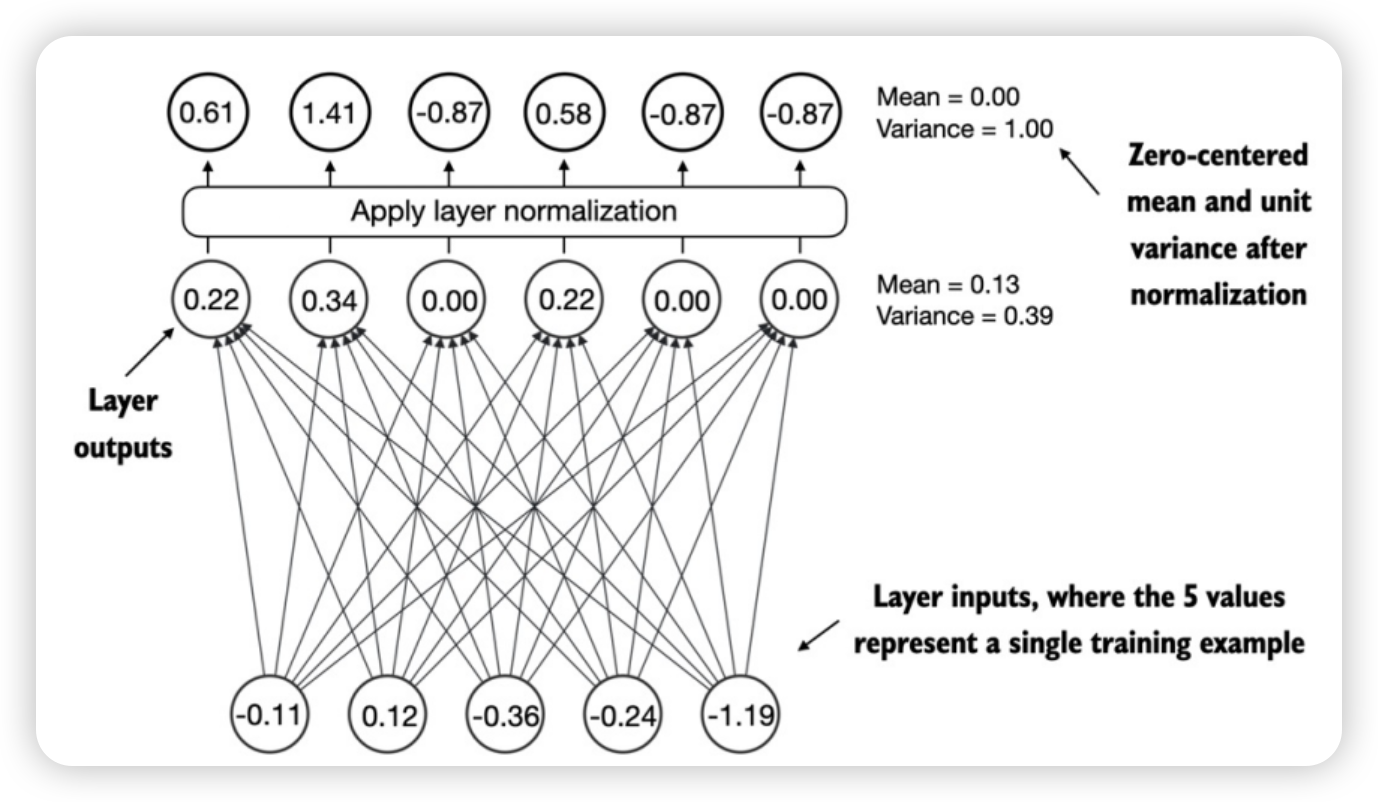
主要思想：调整神经网络层的激活（输出），使其为单位方差（平均值为0，方差为1）。
作用：加快收敛速度，确保一致、可靠的训练。
应用：多头注意模块之前和之后，最终输出层之间。

exp

torch.manual_seed(123)
batch_example = torch.randn(2, 5) # 2 * 5
# 一个 5 * 6 线性层和一个非线性激活函数 ReLU
layer = nn.Sequential(nn.Linear(5, 6), nn.ReLU())
out = layer(batch_example)
print(out.shape)
print(out)

torch.Size([2, 6])
tensor([[0.2260, 0.3470, 0.0000, 0.2216, 0.0000, 0.0000],
        [0.2133, 0.2394, 0.0000, 0.5198, 0.3297, 0.0000]],
       grad_fn=<ReluBackward0>)

# 检查均值 mean 和方差 var

# keepdim保持输出维度与输入维度相同
mean = out.mean(dim=-1, keepdim=True)
var = out.var(dim=-1, keepdim=True)
print("Mean:\n", mean)
print("Variance:\n", var)

Mean:
 tensor([[0.1324],
        [0.2170]], grad_fn=<MeanBackward1>)
Variance:
 tensor([[0.0231],
        [0.0398]], grad_fn=<VarBackward0>)

# 归一化

out_norm = (out - mean) / torch.sqrt(var)
mean = out_norm.mean(dim=-1, keepdim=True)
var = out_norm.var(dim=-1, keepdim=True)

print("Normalized layer outputs:\n", out_norm)
print("Mean:\n", mean)
print("Variance:\n", var)

Normalized layer outputs:
 tensor([[ 0.6159,  1.4126, -0.8719,  0.5872, -0.8719, -0.8719],
        [-0.0189,  0.1121, -1.0876,  1.5173,  0.5647, -1.0876]],
       grad_fn=<DivBackward0>)
Mean:
 tensor([[2.9802e-08],
        [1.9868e-08]], grad_fn=<MeanBackward1>)
Variance:
 tensor([[1.0000],
        [1.0000]], grad_fn=<VarBackward0>)

# 关闭科学记数，提高可读性
torch.set_printoptions(sci_mode=False)

print("Mean:\n", mean)
print("Variance:\n", var)

Mean:
 tensor([[    0.0000],
        [    0.0000]], grad_fn=<MeanBackward1>)
Variance:
 tensor([[1.0000],
        [1.0000]], grad_fn=<VarBackward0>)

DummyLayerNorm:

归一化公式：
$y=\frac{x-E[x]}{\sqrt{Var[x]+\epsilon}}\mathrm{~*~}\gamma+\beta$

$\epsilon$ : eps是小常数，防止分母为0；
两个可训练参数（与输入维度相同）
- $\gamma$ : scale
- $\beta$ : shift

import torch.nn as nn

# 归一化 模块
class LayerNorm(nn.Module):
    def __init__(self, emb_dim):
        super().__init__()
        self.eps = 1e-5
        self.scale = nn.Parameter(torch.ones(emb_dim))
        self.shift = nn.Parameter(torch.zeros(emb_dim))
        
    def forward(self, x):
        mean = x.mean(dim=-1, keepdim=True)
        # unbiased=False 
        # 除以 n 为了与GPT-2的归一化层兼容
        # 有的采用贝塞尔校正，是除以 n-1
        var = x.var(dim=-1, keepdim=True, unbiased=False)
        norm_x = (x - mean) / torch.sqrt(var + self.eps)
        return self.scale * norm_x + self.shift

测试

ln = LayerNorm(emb_dim=5)
out_ln = ln(batch_example)
mean = out_ln.mean(dim=-1, keepdim=True)
var = out_ln.var(dim=-1, unbiased=False, keepdim=True)

print("Mean:\n", mean)
print("Variance:\n", var)

Mean:
 tensor([[    -0.0000],
        [     0.0000]], grad_fn=<MeanBackward1>)
Variance:
 tensor([[1.0000],
        [1.0000]], grad_fn=<VarBackward0>)

GELU activation

激活函数

工作原理

引入非线性：模拟复杂的函数关系
加速训练：区间线性
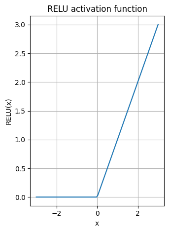
- ReLU正区间线性
防止梯度消失/爆炸：输入值极端梯度接近于零
- Sigmoid
实现稀疏性：减少计算量并提高模型的泛化能力

ReLU函数（整流线性单位函数）

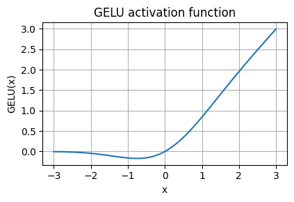
GELU函数（高斯误差线性单元函数）

公式

$\Phi(x)$

其中 $ \Phi(x) $ 是标准高斯分布函数。

$\approx 0.5 \cdot x \cdot (1 + \tanh[\sqrt{(2/\pi)} \cdot (x + 0.044715 \cdot x^3)])$

代码

import torch
from torch import nn

# GELU 激活函数
class GELU(nn.Module):
    def __init__(self):
        super().__init__()
    def forward(self, x):
        return 0.5 * x * (1 + torch.tanh(
            torch.sqrt(torch.tensor(2.0 / torch.pi)) * 
            (x + 0.044715 * torch.pow(x, 3))
        ))

绘制

import matplotlib.pyplot as plt
gelu, relu = GELU(), nn.ReLU()
x = torch.linspace(-3, 3, 100)
y_gelu, y_relu = gelu(x), relu(x)
plt.figure(figsize=(8,3))
for i, (y, label) in enumerate(zip([y_gelu, y_relu], ["GELU", "RELU"]), 1):
    plt.subplot(1, 2, i)
    plt.plot(x, y)
    plt.title(f"{label} activation function")
    plt.xlabel("x")
    plt.ylabel(f"{label}(x)")
    plt.grid(True)
    plt.tight_layout()
    plt.show()

png

SwiGLU（Sigmoid-权重线性单元函数）

Feed forward network

代码 - FeedForward

# 用 GELU 实现一个小型神经网络模块
import torch.nn as nn

class FeedForward(nn.Module):
    def __init__(self, cfg):
        super().__init__()
        # 两个线性层和一个GELU激活函数
        self.layers = nn.Sequential(
            nn.Linear(cfg["emb_dim"], 4 * cfg["emb_dim"]),
            GELU(),
            nn.Linear(4 * cfg["emb_dim"], cfg["emb_dim"]),
        )
 
    def forward(self, x):
        return self.layers(x)

数据流图：

GPT-2的数据流图.png

测试

ffn = FeedForward(GPT_CONFIG_124M)
x = torch.rand(2, 3, 768)
out = ffn(x)
print(out.shape)

torch.Size([2, 3, 768])

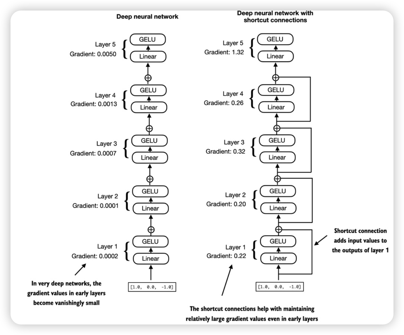
Shortcut connections

图例及实现

import torch.nn as nn
from torch.nn import GELU

class ExampleDeepNeuralNetwork(nn.Module):
    def __init__(self, layer_sizes, use_shortcut):
        super().__init__()
        self.use_shortcut = use_shortcut
        # Sequential 自动顺序执行；
        # ModuleList 手动指定执行；
        self.layers = nn.ModuleList([
            nn.Sequential(nn.Linear(layer_sizes[0], layer_sizes[1]), GELU()),
            nn.Sequential(nn.Linear(layer_sizes[1], layer_sizes[2]), GELU()),
            nn.Sequential(nn.Linear(layer_sizes[2], layer_sizes[3]), GELU()),
            nn.Sequential(nn.Linear(layer_sizes[3], layer_sizes[4]), GELU()),
            nn.Sequential(nn.Linear(layer_sizes[4], layer_sizes[5]), GELU()),
        ])
    def forward(self, x):
        for layer in self.layers:
            layer_output = layer(x)
            if self.use_shortcut and x.shape == layer_output.shape:
                x = x + layer_output
            else:
                x = layer_output
        return x

模拟

# 在模型的反向传递中计算梯度

def print_gradients(model, x):
    output = model(x)
    target = torch.tensor([[0.]])
    
    # 根据目标和输出的接近程度计算损失
    # 模拟模型输出与用户指定目标的接近程度
    loss = nn.MSELoss()
    loss = loss(output, target)
    
    # 反向传播：计算每一层的损失梯度
    loss.backward()
    
    # 迭代权重参数，打印平均绝对梯度
    for name, param in model.named_parameters():
        if "weight" in name:
            # 输出权重的平均绝对梯度
            print(f"{name} has gradinet mean of {param.grad.abs().mean()}")

# 测试 - 不使用快捷连接：

layer_sizes = [3, 3, 3, 3, 3, 1]
sample_input = torch.tensor([[1., 0., -1.]])


torch.manual_seed(123) # 为初始权重指定随机种子以确保可重现性
model_without_shortcut = ExampleDeepNeuralNetwork(
     layer_sizes, use_shortcut=False
)

print_gradients(model_without_shortcut, sample_input)

layers.0.0.weight has gradinet mean of 0.0002017411752603948
layers.1.0.weight has gradinet mean of 0.00012011770741082728
layers.2.0.weight has gradinet mean of 0.0007152436301112175
layers.3.0.weight has gradinet mean of 0.0013988513965159655
layers.4.0.weight has gradinet mean of 0.005049605388194323

梯度从最后一层（layers.4）到第一层（layers.0）逐渐变小 —— 梯度消失。

# 测试 - 使用快捷连接：

torch.manual_seed(123) # 为初始权重指定随机种子以确保可重现性
model_without_shortcut = ExampleDeepNeuralNetwork(
     layer_sizes, use_shortcut=True
)

print_gradients(model_without_shortcut, sample_input)

layers.0.0.weight has gradinet mean of 0.22186797857284546
layers.1.0.weight has gradinet mean of 0.20709273219108582
layers.2.0.weight has gradinet mean of 0.32923877239227295
layers.3.0.weight has gradinet mean of 0.2667772173881531
layers.4.0.weight has gradinet mean of 1.3268063068389893

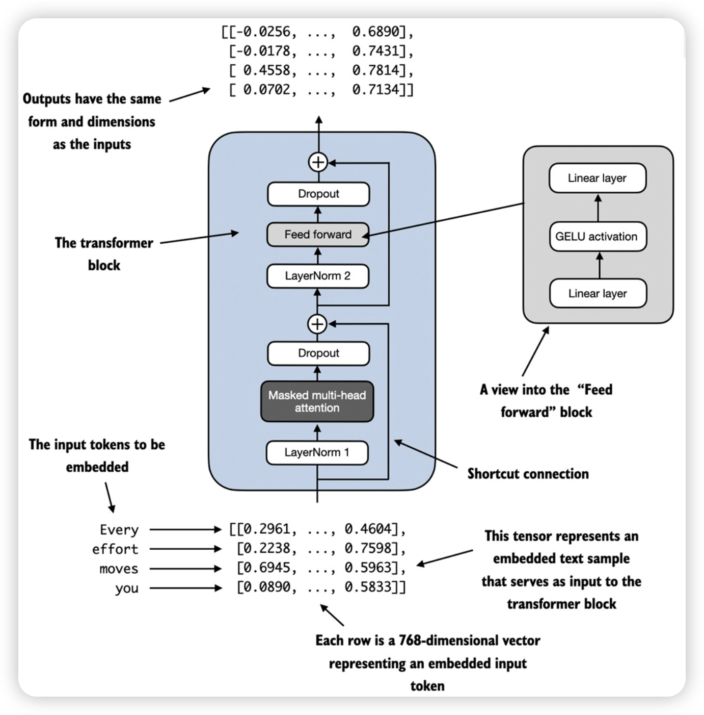
Transformer block

架构图

包括层归一化，多头注意力，Dropout，前馈网络层（GELU 激活函数）和快捷链接

Transformer块示意图.png

代码 - MultiHeadAttention

import torch
import torch.nn as nn

# 多头注意力类
class MultiHeadAttention(nn.Module):
    
    def __init__(self, d_in, d_out, context_length, dropout, num_heads, qkv_bias=False):
        super().__init__()
        assert d_out % num_heads == 0, "d_out must be divisible by num_heads" # A
        self.d_out = d_out
        self.num_heads = num_heads
        self.head_dim = d_out // num_heads
        
        self.W_query = nn.Linear(d_in, d_out, bias=qkv_bias)
        self.W_key = nn.Linear(d_in, d_out, bias=qkv_bias)
        self.W_value = nn.Linear(d_in, d_out, bias=qkv_bias)
        self.out_proj = nn.Linear(d_out, d_out)
        self.dropout = nn.Dropout(dropout)
        self.register_buffer('mask', torch.triu(torch.ones(context_length, context_length), diagonal=1))
        
    def forward(self, x):
        b, num_tokens, d_in = x.shape
        # [(b, num_tokens, d_out)]
        keys = self.W_key(x) 
        queries = self.W_query(x)
        values = self.W_value(x)
        
        # [(b, num_tokens, num_heads, num_dim)]
        keys = keys.view(b, num_tokens, self.num_heads, self.head_dim)
        queries = queries.view(b, num_tokens, self.num_heads, self.head_dim)
        values = values.view(b, num_tokens, self.num_heads, self.head_dim)
        
        # [(b, num_heads, num_tokens, num_dim)]
        keys = keys.transpose(1, 2)
        queries = queries.transpose(1, 2)
        values = values.transpose(1, 2)
        
        # [(b, num_heads, num_tokens, num_tokens)]
        attn_scores = queries @ keys.transpose(2, 3)
        mask_bool = self.mask.bool()[:num_tokens, :num_tokens]
        attn_scores.masked_fill_(mask_bool, -torch.inf)
        attn_weights = torch.softmax(
            attn_scores / keys.shape[-1] ** 0.5, dim=-1)
        attn_weights = self.dropout(attn_weights)
        
        # [(b, num_tokens, num_heads, num_dim)]
        context_vec = (attn_weights @ values).transpose(1, 2)
        # [(b, num_tokens, d_out)]
        context_vec = context_vec.contiguous().view(b, num_tokens, self.d_out)
        context_vec = self.out_proj(context_vec)
        return context_vec

代码 - FeedForward

import torch.nn as nn

# FeedForward 前馈网络块
class FeedForward(nn.Module):
    def __init__(self, cfg):
        super().__init__()
        self.linear1 = nn.Linear(cfg["emb_dim"], cfg["emb_dim"] * 4)
        self.relu = nn.ReLU()
        self.linear2 = nn.Linear(cfg["emb_dim"] * 4, cfg["emb_dim"])
        self.dropout = nn.Dropout(cfg["drop_rate"])
 
    def forward(self, x):
        x = self.relu(self.linear1(x))
        x = self.dropout(x)
        x = self.linear2(x)
        return x

代码 - TransformerBlock

import torch.nn as nn
from torch.nn import LayerNorm

class TransformerBlock(nn.Module):
    def __init__(self, cfg):
        super().__init__()
        self.att = MultiHeadAttention(
            d_in=cfg["emb_dim"],
            d_out=cfg["emb_dim"],
            context_length=cfg["context_length"],
            dropout=cfg["drop_rate"], 
            num_heads=cfg["n_heads"], 
            qkv_bias=cfg["qkv_bias"],
        )
        
        self.ff = FeedForward(cfg)
        self.norm1 = LayerNorm(cfg["emb_dim"])
        self.norm2 = LayerNorm(cfg["emb_dim"])
        self.drop_resid = nn.Dropout(cfg["drop_rate"])
        
    def forward(self, x):
        shortcut = x
        x = self.norm1(x)
        x = self.att(x)
        x = self.drop_resid(x)
        x = x + shortcut
        
        shortcut = x
        x = self.norm2(x)
        x = self.ff(x)
        x = self.drop_resid(x)
        x = x + shortcut
        return x

测试

torch.manual_seed(123)
x = torch.rand(2, 4, 768)
block = TransformerBlock(GPT_CONFIG_124M)
output = block(x)
print("Input shape:", x.shape)
print("Output shape:", output.shape)

Input shape: torch.Size([2, 4, 768])
Output shape: torch.Size([2, 4, 768])