


Part 1:Python Basics with Numpy (optional assignment)
1 - Building basic functions with numpy
Numpy is the main package for scientific computing in Python. It is maintained by a large community (www.numpy.org). In this exercise you will learn several key numpy functions such as np.exp, np.log, and np.reshape. You will need to know how to use these functions for future assignments.
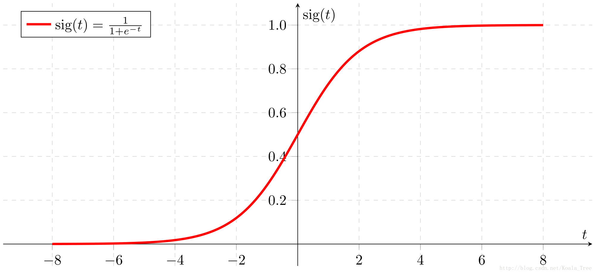
1.1 - sigmoid function, np.exp()
Exercise: Build a function that returns the sigmoid of a real number x. Use math.exp(x) for the exponential function.
Reminder:
sigmoid(x)=11+e−x
is sometimes also known as the logistic function. It is a non-linear function used not only in Machine Learning (Logistic Regression), but also in Deep Learning.
To refer to a function belonging to a specific package you could call it using package_name.function(). Run the code below to see an example with math.exp().
- 1
- 2
- 3
- 4
- 5
- 6
- 7
- 8
- 9
- 10
- 11
- 12
- 13
- 14
- 15
- 16
- 17
- 18
- 19
- 20
- 1
- 1
- 2
Actually, we rarely use the “math” library in deep learning because the inputs of the functions are real numbers. In deep learning we mostly use matrices and vectors. This is why numpy is more useful.
- 1
- 2
- 3
- 1
- 2
- 3
- 4
- 5
- 6
- 7
- 8
- 9
- 10
- 11
- 12
- 13
- 14
- 15
- 16
- 17
- 18
- 19
- 20
In fact, if x=(x1,x2,...,xn) is a row vector then np.exp(x) will apply the exponential function to every element of x. The output will thus be: np.exp(x)=(ex1,ex2,...,exn)
- 1
- 2
- 3
- 4
- 5
- 1
- 2
Furthermore, if x is a vector, then a Python operation such as s=x+3 or s=1x will output s as a vector of the same size as x.
- 1
- 2
- 3
- 1
- 2
Exercise: Implement the sigmoid function using numpy.
Instructions: x could now be either a real number, a vector, or a matrix. The data structures we use in numpy to represent these shapes (vectors, matrices…) are called numpy arrays. You don’t need to know more for now.
- 1
- 2
- 3
- 4
- 5
- 6
- 7
- 8
- 9
- 10
- 11
- 12
- 13
- 14
- 15
- 16
- 17
- 18
- 19
- 20
- 1
- 2
- 1
- 2
1.2 - Sigmoid gradient
Exercise: Implement the function sigmoid_grad() to compute the gradient of the sigmoid function with respect to its input x. The formula is:
You often code this function in two steps:
1. Set s to be the sigmoid of x. You might find your sigmoid(x) function useful.
2. Compute σ′(x)=s(1−s)
- 1
- 2
- 3
- 4
- 5
- 6
- 7
- 8
- 9
- 10
- 11
- 12
- 13
- 14
- 15
- 16
- 17
- 18
- 19
- 20
- 1
- 2
- 1
- 2
1.3 - Reshaping arrays
Two common numpy functions used in deep learning are np.shape and np.reshape().
- X.shape is used to get the shape (dimension) of a matrix/vector X.
- X.reshape(…) is used to reshape X into some other dimension.
For example, in computer science, an image is represented by a 3D array of shape (length,height,depth=3) . However, when you read an image as the input of an algorithm you convert it to a vector of shape (length∗height∗3,1) . In other words, you “unroll”, or reshape, the 3D array into a 1D vector.
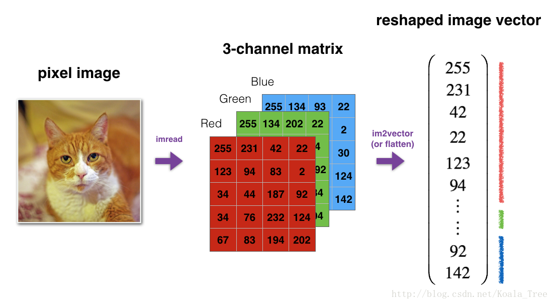
Exercise: Implement image2vector() that takes an input of shape (length, height, 3) and returns a vector of shape (length*height*3, 1). For example, if you would like to reshape an array v of shape (a, b, c) into a vector of shape (a*b,c) you would do:
- 1
- Please don’t hardcode the dimensions of image as a constant. Instead look up the quantities you need with
image.shape[0], etc.
- 1
- 2
- 3
- 4
- 5
- 6
- 7
- 8
- 9
- 10
- 11
- 12
- 13
- 14
- 15
- 1
- 2
- 3
- 4
- 5
- 6
- 7
- 8
- 9
- 10
- 11
- 12
- 13
- 14
- 1
- 2
- 3
- 4
- 5
- 6
- 7
- 8
- 9
- 10
- 11
- 12
- 13
- 14
- 15
- 16
- 17
- 18
- 19
1.4 - Normalizing rows
Another common technique we use in Machine Learning and Deep Learning is to normalize our data. It often leads to a better performance because gradient descent converges faster after normalization. Here, by normalization we mean changing x to x∥x∥ (dividing each row vector of x by its norm).
For example, if
Exercise: Implement normalizeRows() to normalize the rows of a matrix. After applying this function to an input matrix x, each row of x should be a vector of unit length (meaning length 1).
- 1
- 2
- 3
- 4
- 5
- 6
- 7
- 8
- 9
- 10
- 11
- 12
- 13
- 14
- 15
- 16
- 17
- 18
- 19
- 20
- 21
- 22
- 1
- 2
- 3
- 4
- 1
- 2
- 3
Note:
In normalizeRows(), you can try to print the shapes of x_norm and x, and then rerun the assessment. You’ll find out that they have different shapes. This is normal given that x_norm takes the norm of each row of x. So x_norm has the same number of rows but only 1 column. So how did it work when you divided x by x_norm? This is called broadcasting and we’ll talk about it now!
1.5 - Broadcasting and the softmax function
A very important concept to understand in numpy is “broadcasting”. It is very useful for performing mathematical operations between arrays of different shapes. For the full details on broadcasting, you can read the official broadcasting documentation.
Exercise: Implement a softmax function using numpy. You can think of softmax as a normalizing function used when your algorithm needs to classify two or more classes. You will learn more about softmax in the second course of this specialization.
Instructions:
-
-
for a matrix x∈Rm×n, xij maps to the element in the ith row and jth column of x, thus we have:
softmax(x)=softmax⎡⎣⎢⎢⎢⎢⎢x11x21⋮xm1x12x22⋮xm2x13x23⋮xm3……⋱…x1nx2n⋮xmn⎤⎦⎥⎥⎥⎥⎥=⎡⎣⎢⎢⎢⎢⎢⎢⎢⎢⎢⎢⎢⎢⎢ex11∑jex1jex21∑jex2j⋮exm1∑jexmjex12∑jex1jex22∑jex2j⋮exm2∑jexmjex13∑jex1jex23∑jex2j⋮exm3∑jexmj……⋱…ex1n∑jex1jex2n∑jex2j⋮exmn∑jexmj⎤⎦⎥⎥⎥⎥⎥⎥⎥⎥⎥⎥⎥⎥⎥=⎛⎝⎜⎜⎜⎜softmax(first row of x)softmax(second row of x)...softmax(last row of x)⎞⎠⎟⎟⎟⎟
- 1
- 2
- 3
- 4
- 5
- 6
- 7
- 8
- 9
- 10
- 11
- 12
- 13
- 14
- 15
- 16
- 17
- 18
- 19
- 20
- 21
- 22
- 23
- 24
- 25
- 26
- 27
- 1
- 2
- 3
- 4
- 1
- 2
- 3
- 4
- 5
Note:
- If you print the shapes of x_exp, x_sum and s above and rerun the assessment cell, you will see that x_sum is of shape (2,1) while x_exp and s are of shape (2,5). x_exp/x_sum works due to python broadcasting.
What you need to remember:
- np.exp(x) works for any np.array x and applies the exponential function to every coordinate
- the sigmoid function and its gradient
- image2vector is commonly used in deep learning
- np.reshape is widely used. In the future, you’ll see that keeping your matrix/vector dimensions straight will go toward eliminating a lot of bugs.
- numpy has efficient built-in functions
- broadcasting is extremely useful
2) Vectorization
In deep learning, you deal with very large datasets. Hence, a non-computationally-optimal function can become a huge bottleneck in your algorithm and can result in a model that takes ages to run. To make sure that your code is computationally efficient, you will use vectorization. For example, try to tell the difference between the following implementations of the dot/outer/elementwise product.
- 1
- 2
- 3
- 4
- 5
- 6
- 7
- 8
- 9
- 10
- 11
- 12
- 13
- 14
- 15
- 16
- 17
- 18
- 19
- 20
- 21
- 22
- 23
- 24
- 25
- 26
- 27
- 28
- 29
- 30
- 31
- 32
- 33
- 34
- 35
- 36
- 37
- 38
- 39
- 1
- 2
- 3
- 4
- 5
- 6
- 7
- 8
- 9
- 10
- 11
- 12
- 13
- 14
- 15
- 16
- 17
- 18
- 19
- 20
- 21
- 22
- 23
- 24
- 25
- 26
- 27
- 28
- 29
- 30
- 31
- 32
- 33
- 34
- 35
- 36
- 37
- 38
- 1
- 2
- 3
- 4
- 5
- 6
- 7
- 8
- 9
- 10
- 11
- 12
- 13
- 14
- 15
- 16
- 17
- 18
- 19
- 20
- 21
- 22
- 23
- 24
- 25
- 26
- 1
- 2
- 3
- 4
- 5
- 6
- 7
- 8
- 9
- 10
- 11
- 12
- 13
- 14
- 15
- 16
- 17
- 18
- 19
- 20
- 21
- 22
- 23
As you may have noticed, the vectorized implementation is much cleaner and more efficient. For bigger vectors/matrices, the differences in running time become even bigger.
Note that np.dot() performs a matrix-matrix or matrix-vector multiplication. This is different from np.multiply() and the * operator (which is equivalent to .* in Matlab/Octave), which performs an element-wise multiplication.
2.1 Implement the L1 and L2 loss functions
Exercise: Implement the numpy vectorized version of the L1 loss. You may find the function abs(x) (absolute value of x) useful.
Reminder:
- The loss is used to evaluate the performance of your model. The bigger your loss is, the more different your predictions (
y^
) are from the true values (
y
). In deep learning, you use optimization algorithms like Gradient Descent to train your model and to minimize the cost.
- L1 loss is defined as:
- 1
- 2
- 3
- 4
- 5
- 6
- 7
- 8
- 9
- 10
- 11
- 12
- 13
- 14
- 15
- 16
- 17
- 1
- 2
- 3
- 1
- 2
Exercise: Implement the numpy vectorized version of the L2 loss. There are several way of implementing the L2 loss but you may find the function np.dot() useful. As a reminder, if
x=[x1,x2,...,xn]
, then np.dot(x,x) =
∑nj=0x2j
.
- L2 loss is defined as
- 1
- 2
- 3
- 4
- 5
- 6
- 7
- 8
- 9
- 10
- 11
- 12
- 13
- 14
- 15
- 16
- 17
- 1
- 2
- 3
- 1
- 2
What to remember:
- Vectorization is very important in deep learning. It provides computational efficiency and clarity.
- You have reviewed the L1 and L2 loss.
- You are familiar with many numpy functions such as np.sum, np.dot, np.multiply, np.maximum, etc…
Part 2: Logistic Regression with a Neural Network mindset
You will learn to:
- Build the general architecture of a learning algorithm, including:
- Initializing parameters
- Calculating the cost function and its gradient
- Using an optimization algorithm (gradient descent)
- Gather all three functions above into a main model function, in the right order.
1 - Packages
First, let’s run the cell below to import all the packages that you will need during this assignment.
- numpy is the fundamental package for scientific computing with Python.
- h5py is a common package to interact with a dataset that is stored on an H5 file.
- matplotlib is a famous library to plot graphs in Python.
- PIL and scipy are used here to test your model with your own picture at the end.
- 1
- 2
- 3
- 4
- 5
- 6
- 7
- 8
- 9
2 - Overview of the Problem set
Problem Statement: You are given a dataset (“data.h5”) containing:
- a training set of m_train images labeled as cat (y=1) or non-cat (y=0)
- a test set of m_test images labeled as cat or non-cat
- each image is of shape (num_px, num_px, 3) where 3 is for the 3 channels (RGB). Thus, each image is square (height = num_px) and (width = num_px).
You will build a simple image-recognition algorithm that can correctly classify pictures as cat or non-cat.
Let’s get more familiar with the dataset. Load the data by running the following code.
- 1
- 2
We added “_orig” at the end of image datasets (train and test) because we are going to preprocess them. After preprocessing, we will end up with train_set_x and test_set_x (the labels train_set_y and test_set_y don’t need any preprocessing).
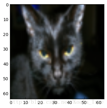
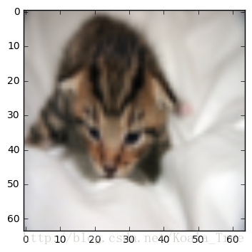
Each line of your train_set_x_orig and test_set_x_orig is an array representing an image. You can visualize an example by running the following code. Feel free also to change the index value and re-run to see other images.
- 1
- 2
- 3
- 4
- 1
- 2
Many software bugs in deep learning come from having matrix/vector dimensions that don’t fit. If you can keep your matrix/vector dimensions straight you will go a long way toward eliminating many bugs.
Exercise: Find the values for:
- m_train (number of training examples)
- m_test (number of test examples)
- num_px (= height = width of a training image)
Remember that train_set_x_orig is a numpy-array of shape (m_train, num_px, num_px, 3). For instance, you can access m_train by writing train_set_x_orig.shape[0].
- 1
- 2
- 3
- 4
- 5
- 6
- 7
- 8
- 9
- 10
- 11
- 12
- 13
- 14
- 1
- 2
- 3
- 4
- 5
- 6
- 7
- 8
- 9
For convenience, you should now reshape images of shape (num_px, num_px, 3) in a numpy-array of shape (num_px ∗ num_px ∗ 3, 1). After this, our training (and test) dataset is a numpy-array where each column represents a flattened image. There should be m_train (respectively m_test) columns.
Exercise: Reshape the training and test data sets so that images of size (num_px, num_px, 3) are flattened into single vectors of shape (num_px ∗ num_px ∗ 3, 1).
A trick when you want to flatten a matrix X of shape (a,b,c,d) to a matrix X_flatten of shape (b ∗ c ∗ d, a) is to use:
- 1
- 1
- 2
- 3
- 4
- 5
- 6
- 7
- 8
- 9
- 10
- 11
- 12
- 1
- 2
- 3
- 4
- 5
- 6
To represent color images, the red, green and blue channels (RGB) must be specified for each pixel, and so the pixel value is actually a vector of three numbers ranging from 0 to 255.
One common preprocessing step in machine learning is to center and standardize your dataset, meaning that you substract the mean of the whole numpy array from each example, and then divide each example by the standard deviation of the whole numpy array. But for picture datasets, it is simpler and more convenient and works almost as well to just divide every row of the dataset by 255 (the maximum value of a pixel channel).
Let’s standardize our dataset.
- 1
- 2
What you need to remember:
Common steps for pre-processing a new dataset are:
- Figure out the dimensions and shapes of the problem (m_train, m_test, num_px, …)
- Reshape the datasets such that each example is now a vector of size (num_px * num_px * 3, 1)
- “Standardize” the data
3 - General Architecture of the learning algorithm
It’s time to design a simple algorithm to distinguish cat images from non-cat images.
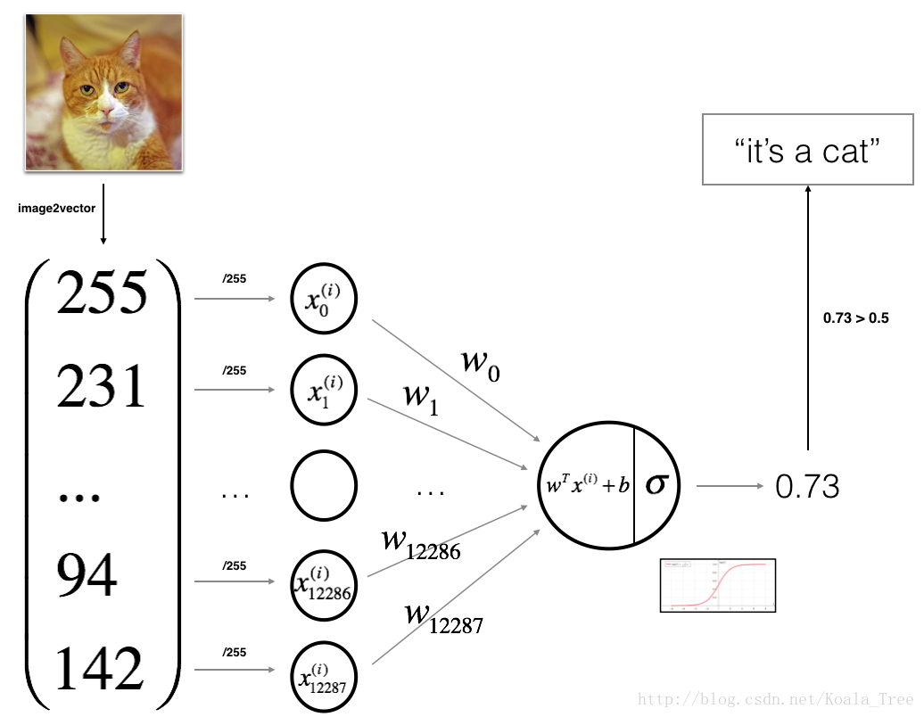
You will build a Logistic Regression, using a Neural Network mindset. The following Figure explains why Logistic Regression is actually a very simple Neural Network!
Mathematical expression of the algorithm:
For one example
x(i)
:
The cost is then computed by summing over all training examples:
Key steps:
In this exercise, you will carry out the following steps:
- Initialize the parameters of the model
- Learn the parameters for the model by minimizing the cost
- Use the learned parameters to make predictions (on the test set)
- Analyse the results and conclude
4 - Building the parts of our algorithm ##
The main steps for building a Neural Network are:
1. Define the model structure (such as number of input features)
2. Initialize the model’s parameters
3. Loop:
- Calculate current loss (forward propagation)
- Calculate current gradient (backward propagation)
- Update parameters (gradient descent)
You often build 1-3 separately and integrate them into one function we call model().
4.1 - Helper functions
Exercise: Using your code from “Python Basics”, implement sigmoid(). As you’ve seen in the figure above, you need to compute
sigmoid(wTx+b)=11+e−(wTx+b)
to make predictions. Use np.exp().
- 1
- 2
- 3
- 4
- 5
- 6
- 7
- 8
- 9
- 10
- 11
- 12
- 13
- 14
- 15
- 16
- 17
- 18
- 1
- 1
- 2
4.2 - Initializing parameters
Exercise: Implement parameter initialization in the cell below. You have to initialize w as a vector of zeros. If you don’t know what numpy function to use, look up np.zeros() in the Numpy library’s documentation.
- 1
- 2
- 3
- 4
- 5
- 6
- 7
- 8
- 9
- 10
- 11
- 12
- 13
- 14
- 15
- 16
- 17
- 18
- 19
- 20
- 21
- 22
- 23
- 1
- 2
- 3
- 4
- 1
- 2
- 3
- 4
For image inputs, w will be of shape (num_px × num_px × 3, 1).
4.3 - Forward and Backward propagation
Now that your parameters are initialized, you can do the “forward” and “backward” propagation steps for learning the parameters.
Exercise: Implement a function propagate() that computes the cost function and its gradient.
Hints:
Forward Propagation:
- You get X
- You compute
A=σ(wTX+b)=(a(0),a(1),...,a(m−1),a(m))
- You calculate the cost function:
J=−1m∑mi=1y(i)log(a(i))+(1−y(i))log(1−a(i))
Here are the two formulas you will be using:
- 1
- 2
- 3
- 4
- 5
- 6
- 7
- 8
- 9
- 10
- 11
- 12
- 13
- 14
- 15
- 16
- 17
- 18
- 19
- 20
- 21
- 22
- 23
- 24
- 25
- 26
- 27
- 28
- 29
- 30
- 31
- 32
- 33
- 34
- 35
- 36
- 37
- 38
- 39
- 40
- 41
- 42
- 43
- 44
- 1
- 2
- 3
- 4
- 5
- 1
- 2
- 3
- 4
- 5
d) Optimization
- You have initialized your parameters.
- You are also able to compute a cost function and its gradient.
- Now, you want to update the parameters using gradient descent.
Exercise: Write down the optimization function. The goal is to learn w and b by minimizing the cost function J . For a parameter θ , the update rule is θ=θ−α dθ , where α is the learning rate.
- 1
- 2
- 3
- 4
- 5
- 6
- 7
- 8
- 9
- 10
- 11
- 12
- 13
- 14
- 15
- 16
- 17
- 18
- 19
- 20
- 21
- 22
- 23
- 24
- 25
- 26
- 27
- 28
- 29
- 30
- 31
- 32
- 33
- 34
- 35
- 36
- 37
- 38
- 39
- 40
- 41
- 42
- 43
- 44
- 45
- 46
- 47
- 48
- 49
- 50
- 51
- 52
- 53
- 54
- 55
- 56
- 57
- 58
- 59
- 60
- 61
- 1
- 2
- 3
- 4
- 5
- 6
- 1
- 2
- 3
- 4
- 5
- 6
- 7
Exercise: The previous function will output the learned w and b. We are able to use w and b to predict the labels for a dataset X. Implement the predict() function. There is two steps to computing predictions:
-
Calculate Y^=A=σ(wTX+b)
-
Convert the entries of a into 0 (if activation <= 0.5) or 1 (if activation > 0.5), stores the predictions in a vector
Y_prediction. If you wish, you can use anif/elsestatement in aforloop (though there is also a way to vectorize this).
- 1
- 2
- 3
- 4
- 5
- 6
- 7
- 8
- 9
- 10
- 11
- 12
- 13
- 14
- 15
- 16
- 17
- 18
- 19
- 20
- 21
- 22
- 23
- 24
- 25
- 26
- 27
- 28
- 29
- 30
- 31
- 32
- 33
- 34
- 35
- 36
- 37
- 1
- 2
- 3
- 4
- 1
- 2
What to remember:
You’ve implemented several functions that:
- Initialize (w,b)
- Optimize the loss iteratively to learn parameters (w,b):
- computing the cost and its gradient
- updating the parameters using gradient descent
- Use the learned (w,b) to predict the labels for a given set of examples
5 - Merge all functions into a model
You will now see how the overall model is structured by putting together all the building blocks (functions implemented in the previous parts) together, in the right order.
Exercise: Implement the model function. Use the following notation:
- Y_prediction for your predictions on the test set
- Y_prediction_train for your predictions on the train set
- w, costs, grads for the outputs of optimize()
- 1
- 2
- 3
- 4
- 5
- 6
- 7
- 8
- 9
- 10
- 11
- 12
- 13
- 14
- 15
- 16
- 17
- 18
- 19
- 20
- 21
- 22
- 23
- 24
- 25
- 26
- 27
- 28
- 29
- 30
- 31
- 32
- 33
- 34
- 35
- 36
- 37
- 38
- 39
- 40
- 41
- 42
- 43
- 44
- 45
- 46
- 47
- 48
- 49
- 50
- 51
Run the following cell to train your model.
- 1
- 1
- 2
- 3
- 4
- 5
- 6
- 7
- 8
- 9
- 10
- 11
- 12
- 13
- 14
- 15
- 16
- 17
- 18
- 19
- 20
- 21
- 22
- 23
Comment: Training accuracy is close to 100%. This is a good sanity check: your model is working and has high enough capacity to fit the training data. Test error is 68%. It is actually not bad for this simple model, given the small dataset we used and that logistic regression is a linear classifier. But no worries, you’ll build an even better classifier next week!
Also, you see that the model is clearly overfitting the training data. Later in this specialization you will learn how to reduce overfitting, for example by using regularization. Using the code below (and changing the index variable) you can look at predictions on pictures of the test set.
- 1
- 2
- 3
- 4
- 1
- 2
Let’s also plot the cost function and the gradients.
- 1
- 2
- 3
- 4
- 5
- 6
- 7
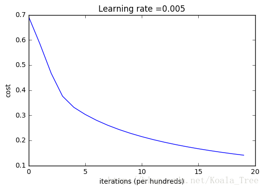
Interpretation:
You can see the cost decreasing. It shows that the parameters are being learned. However, you see that you could train the model even more on the training set. Try to increase the number of iterations in the cell above and rerun the cells. You might see that the training set accuracy goes up, but the test set accuracy goes down. This is called overfitting.
6 - Further analysis (optional/ungraded exercise)
Congratulations on building your first image classification model. Let’s analyze it further, and examine possible choices for the learning rate α .
Choice of learning rate
Reminder:
In order for Gradient Descent to work you must choose the learning rate wisely. The learning rate
α
determines how rapidly we update the parameters. If the learning rate is too large we may “overshoot” the optimal value. Similarly, if it is too small we will need too many iterations to converge to the best values. That’s why it is crucial to use a well-tuned learning rate.
Let’s compare the learning curve of our model with several choices of learning rates. Run the cell below. This should take about 1 minute. Feel free also to try different values than the three we have initialized the learning_rates variable to contain, and see what happens.
- 1
- 2
- 3
- 4
- 5
- 6
- 7
- 8
- 9
- 10
- 11
- 12
- 13
- 14
- 15
- 16
- 17
- 1
- 2
- 3
- 4
- 5
- 6
- 7
- 8
- 9
- 10
- 11
- 12
- 13
- 14
- 15
- 16
- 17
- 18
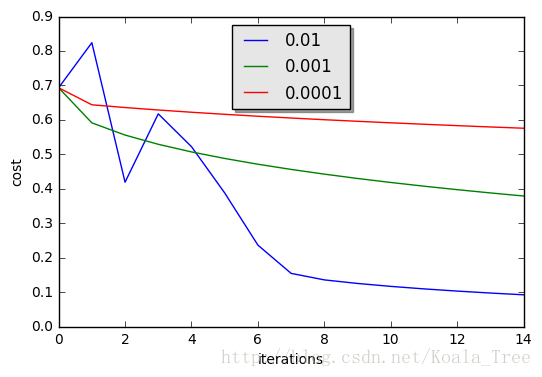
Interpretation:
- Different learning rates give different costs and thus different predictions results.
- If the learning rate is too large (0.01), the cost may oscillate up and down. It may even diverge (though in this example, using 0.01 still eventually ends up at a good value for the cost).
- A lower cost doesn’t mean a better model. You have to check if there is possibly overfitting. It happens when the training accuracy is a lot higher than the test accuracy.
- In deep learning, we usually recommend that you:
- Choose the learning rate that better minimizes the cost function.
- If your model overfits, use other techniques to reduce overfitting. (We’ll talk about this in later videos.)
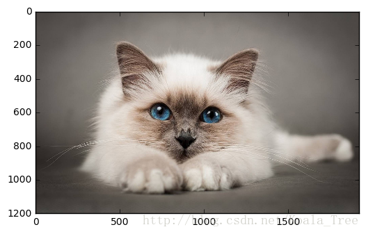
7 - Test with your own image (optional/ungraded exercise)
Congratulations on finishing this assignment. You can use your own image and see the output of your model. To do that:
1. Click on “File” in the upper bar of this notebook, then click “Open” to go on your Coursera Hub.
2. Add your image to this Jupyter Notebook’s directory, in the “images” folder
3. Change your image’s name in the following code
4. Run the code and check if the algorithm is right (1 = cat, 0 = non-cat)!
- 1
- 2
- 3
- 4
- 5
- 6
- 7
- 8
- 9
- 10
- 11
- 12
- 1
- 2
What to remember from this assignment:
1. Preprocessing the dataset is important.
2. You implemented each function separately: initialize(), propagate(), optimize(). Then you built a model().
3. Tuning the learning rate (which is an example of a “hyperparameter”) can make a big difference to the algorithm. You will see more examples of this later in this course!


 1万+
1万+

 被折叠的 条评论
为什么被折叠?
被折叠的 条评论
为什么被折叠?
 到【灌水乐园】发言


