吴恩达深度学习编程作业（2-1）- Initialization & Regularization & Gradient Checking

最新推荐文章于 2024-03-12 19:00:31 发布

大树先生的博客

最新推荐文章于 2024-03-12 19:00:31 发布

阅读量1.4w

点赞数 18

分类专栏：吴恩达深度学习编程作业文章标签：深度学习改善深层神经网络超参数正则化梯度检验

本文链接：https://blog.csdn.net/Koala_Tree/article/details/78137306

版权

吴恩达深度学习编程作业专栏收录该内容

17 篇文章 70 订阅

订阅专栏

吴恩达Coursera课程 DeepLearning.ai 编程作业系列，本文为《改善深层神经网络：超参数调试、正则化以及优化》部分的第四周“深度学习的实践方面”的课程作业，同时增加了一些辅助的测试函数。

另外，本节课程笔记在此：《吴恩达Coursera深度学习课程 DeepLearning.ai 提炼笔记（2-1）– 深度学习的实践方面》，如有任何建议和问题，欢迎留言。

You can get the support code and datasets from here for all the following parts.

Part 1：Initialization

A well chosen initialization can:
- Speed up the convergence of gradient descent
- Increase the odds of gradient descent converging to a lower training (and generalization) error

To get started, run the following cell to load the packages and the planar dataset you will try to classify.

import numpy as np
import matplotlib.pyplot as plt
import sklearn
import sklearn.datasets
from init_utils import sigmoid, relu, compute_loss, forward_propagation, backward_propagation
from init_utils import update_parameters, predict, load_dataset, plot_decision_boundary, predict_dec

%matplotlib inline
plt.rcParams['figure.figsize'] = (7.0, 4.0) # set default size of plots
plt.rcParams['image.interpolation'] = 'nearest'
plt.rcParams['image.cmap'] = 'gray'

# load image dataset: blue/red dots in circles
train_X, train_Y, test_X, test_Y = load_dataset()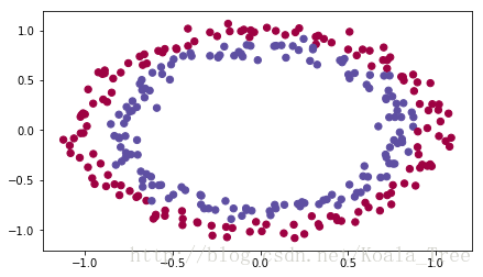

There are some import function：

def sigmoid(x):
    """
    Compute the sigmoid of x

    Arguments:
    x -- A scalar or numpy array of any size.

    Return:
    s -- sigmoid(x)
    """
    s = 1/(1+np.exp(-x))
    return s


def relu(x):
    """
    Compute the relu of x

    Arguments:
    x -- A scalar or numpy array of any size.

    Return:
    s -- relu(x)
    """
    s = np.maximum(0,x)

    return s


def compute_loss(a3, Y):

    """
    Implement the loss function

    Arguments:
    a3 -- post-activation, output of forward propagation
    Y -- "true" labels vector, same shape as a3

    Returns:
    loss - value of the loss function
    """

    m = Y.shape[1]
    logprobs = np.multiply(-np.log(a3),Y) + np.multiply(-np.log(1 - a3), 1 - Y)
    loss = 1./m * np.nansum(logprobs)

    return loss

def forward_propagation(X, parameters):
    """
    Implements the forward propagation (and computes the loss) presented in Figure 2.

    Arguments:
    X -- input dataset, of shape (input size, number of examples)
    Y -- true "label" vector (containing 0 if cat, 1 if non-cat)
    parameters -- python dictionary containing your parameters "W1", "b1", "W2", "b2", "W3", "b3":
                    W1 -- weight matrix of shape ()
                    b1 -- bias vector of shape ()
                    W2 -- weight matrix of shape ()
                    b2 -- bias vector of shape ()
                    W3 -- weight matrix of shape ()
                    b3 -- bias vector of shape ()

    Returns:
    loss -- the loss function (vanilla logistic loss)
    """

    # retrieve parameters
    W1 = parameters["W1"]
    b1 = parameters["b1"]
    W2 = parameters["W2"]
    b2 = parameters["b2"]
    W3 = parameters["W3"]
    b3 = parameters["b3"]

    # LINEAR -> RELU -> LINEAR -> RELU -> LINEAR -> SIGMOID
    z1 = np.dot(W1, X) + b1
    a1 = relu(z1)
    z2 = np.dot(W2, a1) + b2
    a2 = relu(z2)
    z3 = np.dot(W3, a2) + b3
    a3 = sigmoid(z3)

    cache = (z1, a1, W1, b1, z2, a2, W2, b2, z3, a3, W3, b3)

    return a3, cache


def backward_propagation(X, Y, cache):
    """
    Implement the backward propagation presented in figure 2.

    Arguments:
    X -- input dataset, of shape (input size, number of examples)
    Y -- true "label" vector (containing 0 if cat, 1 if non-cat)
    cache -- cache output from forward_propagation()

    Returns:
    gradients -- A dictionary with the gradients with respect to each parameter, activation and pre-activation variables
    """
    m = X.shape[1]
    (z1, a1, W1, b1, z2, a2, W2, b2, z3, a3, W3, b3) = cache

    dz3 = 1./m * (a3 - Y)
    dW3 = np.dot(dz3, a2.T)
    db3 = np.sum(dz3, axis=1, keepdims = True)

    da2 = np.dot(W3.T, dz3)
    dz2 = np.multiply(da2, np.int64(a2 > 0))
    dW2 = np.dot(dz2, a1.T)
    db2 = np.sum(dz2, axis=1, keepdims = True)

    da1 = np.dot(W2.T, dz2)
    dz1 = np.multiply(da1, np.int64(a1 > 0))
    dW1 = np.dot(dz1, X.T)
    db1 = np.sum(dz1, axis=1, keepdims = True)

    gradients = {"dz3": dz3, "dW3": dW3, "db3": db3,
                 "da2": da2, "dz2": dz2, "dW2": dW2, "db2": db2,
                 "da1": da1, "dz1": dz1, "dW1": dW1, "db1": db1}

    return gradients


def update_parameters(parameters, grads, learning_rate):
    """
    Update parameters using gradient descent

    Arguments:
    parameters -- python dictionary containing your parameters 
    grads -- python dictionary containing your gradients, output of n_model_backward

    Returns:
    parameters -- python dictionary containing your updated parameters 
                  parameters['W' + str(i)] = ... 
                  parameters['b' + str(i)] = ...
    """

    L = len(parameters) // 2 # number of layers in the neural networks

    # Update rule for each parameter
    for k in range(L):
        parameters["W" + str(k+1)] = parameters["W" + str(k+1)] - learning_rate * grads["dW" + str(k+1)]
        parameters["b" + str(k+1)] = parameters["b" + str(k+1)] - learning_rate * grads["db" + str(k+1)]

    return parameters


def predict(X, y, parameters):
    """
    This function is used to predict the results of a  n-layer neural network.

    Arguments:
    X -- data set of examples you would like to label
    parameters -- parameters of the trained model

    Returns:
    p -- predictions for the given dataset X
    """

    m = X.shape[1]
    p = np.zeros((1,m), dtype = np.int)

    # Forward propagation
    a3, caches = forward_propagation(X, parameters)

    # convert probas to 0/1 predictions
    for i in range(0, a3.shape[1]):
        if a3[0,i] > 0.5:
            p[0,i] = 1
        else:
            p[0,i] = 0

    # print results
    print("Accuracy: "  + str(np.mean((p[0,:] == y[0,:]))))

    return p


def load_dataset():
    np.random.seed(1)
    train_X, train_Y = sklearn.datasets.make_circles(n_samples=300, noise=.05)
    np.random.seed(2)
    test_X, test_Y = sklearn.datasets.make_circles(n_samples=100, noise=.05)
    # Visualize the data
    plt.scatter(train_X[:, 0], train_X[:, 1], c=train_Y, s=40, cmap=plt.cm.Spectral);
    train_X = train_X.T
    train_Y = train_Y.reshape((1, train_Y.shape[0]))
    test_X = test_X.T
    test_Y = test_Y.reshape((1, test_Y.shape[0]))
    return train_X, train_Y, test_X, test_Y


def plot_decision_boundary(model, X, y):
    # Set min and max values and give it some padding
    x_min, x_max = X[0, :].min() - 1, X[0, :].max() + 1
    y_min, y_max = X[1, :].min() - 1, X[1, :].max() + 1
    h = 0.01
    # Generate a grid of points with distance h between them
    xx, yy = np.meshgrid(np.arange(x_min, x_max, h), np.arange(y_min, y_max, h))
    # Predict the function value for the whole grid
    Z = model(np.c_[xx.ravel(), yy.ravel()])
    Z = Z.reshape(xx.shape)
    # Plot the contour and training examples
    plt.contourf(xx, yy, Z, cmap=plt.cm.Spectral)
    plt.ylabel('x2')
    plt.xlabel('x1')
    plt.scatter(X[0, :], X[1, :], c=y, cmap=plt.cm.Spectral)
    plt.show()


def predict_dec(parameters, X):
    """
    Used for plotting decision boundary.

    Arguments:
    parameters -- python dictionary containing your parameters 
    X -- input data of size (m, K)

    Returns
    predictions -- vector of predictions of our model (red: 0 / blue: 1)
    """

    # Predict using forward propagation and a classification threshold of 0.5
    a3, cache = forward_propagation(X, parameters)
    predictions = (a3>0.5)
    return predictions

You would like a classifier to separate the blue dots from the red dots.

1 - Neural Network model

You will use a 3-layer neural network (already implemented for you). Here are the initialization methods you will experiment with:
- Zeros initialization – setting initialization = "zeros" in the input argument.
- Random initialization – setting initialization = "random" in the input argument. This initializes the weights to large random values.
- He initialization – setting initialization = "he" in the input argument. This initializes the weights to random values scaled according to a paper by He et al., 2015.

Instructions: Please quickly read over the code below, and run it. In the next part you will implement the three initialization methods that this model() calls.

def model(X, Y, learning_rate = 0.01, num_iterations = 15000, print_cost = True, initialization = "he"):
    """
    Implements a three-layer neural network: LINEAR->RELU->LINEAR->RELU->LINEAR->SIGMOID.

    Arguments:
    X -- input data, of shape (2, number of examples)
    Y -- true "label" vector (containing 0 for red dots; 1 for blue dots), of shape (1, number of examples)
    learning_rate -- learning rate for gradient descent 
    num_iterations -- number of iterations to run gradient descent
    print_cost -- if True, print the cost every 1000 iterations
    initialization -- flag to choose which initialization to use ("zeros","random" or "he")

    Returns:
    parameters -- parameters learnt by the model
    """

    grads = {}
    costs = [] # to keep track of the loss
    m = X.shape[1] # number of examples
    layers_dims = [X.shape[0], 10, 5, 1]

    # Initialize parameters dictionary.
    if initialization == "zeros":
        parameters = initialize_parameters_zeros(layers_dims)
    elif initialization == "random":
        parameters = initialize_parameters_random(layers_dims)
    elif initialization == "he":
        parameters = initialize_parameters_he(layers_dims)

    # Loop (gradient descent)

    for i in range(0, num_iterations):

        # Forward propagation: LINEAR -> RELU -> LINEAR -> RELU -> LINEAR -> SIGMOID.
        a3, cache = forward_propagation(X, parameters)

        # Loss
        cost = compute_loss(a3, Y)

        # Backward propagation.
        grads = backward_propagation(X, Y, cache)

        # Update parameters.
        parameters = update_parameters(parameters, grads, learning_rate)

        # Print the loss every 1000 iterations
        if print_cost and i % 1000 == 0:
            print("Cost after iteration {}: {}".format(i, cost))
            costs.append(cost)

    # plot the loss
    plt.plot(costs)
    plt.ylabel('cost')
    plt.xlabel('iterations (per hundreds)')
    plt.title("Learning rate =" + str(learning_rate))
    plt.show()

    return parameters

2 - Zero initialization

There are two types of parameters to initialize in a neural network:
- the weight matrices $(W^{[1]}, W^{[2]}, W^{[3]}, ..., W^{[L-1]}, W^{[L]})$
- the bias vectors $(b^{[1]}, b^{[2]}, b^{[3]}, ..., b^{[L-1]}, b^{[L]})$

Exercise: Implement the following function to initialize all parameters to zeros. You’ll see later that this does not work well since it fails to “break symmetry”, but lets try it anyway and see what happens. Use np.zeros((..,..)) with the correct shapes.

# GRADED FUNCTION: initialize_parameters_zeros 

def initialize_parameters_zeros(layers_dims):
    """
    Arguments:
    layer_dims -- python array (list) containing the size of each layer.

    Returns:
    parameters -- python dictionary containing your parameters "W1", "b1", ..., "WL", "bL":
                    W1 -- weight matrix of shape (layers_dims[1], layers_dims[0])
                    b1 -- bias vector of shape (layers_dims[1], 1)
                    ...
                    WL -- weight matrix of shape (layers_dims[L], layers_dims[L-1])
                    bL -- bias vector of shape (layers_dims[L], 1)
    """

    parameters = {}
    L = len(layers_dims)            # number of layers in the network

    for l in range(1, L):
        ### START CODE HERE ### (≈ 2 lines of code)
        parameters['W' + str(l)] = np.zeros((layers_dims[l],layers_dims[l-1]))
        parameters['b' + str(l)] = np.zeros((layers_dims[l],1))
        ### END CODE HERE ###
    return parameters

parameters = initialize_parameters_zeros([3,2,1])
print("W1 = " + str(parameters["W1"]))
print("b1 = " + str(parameters["b1"]))
print("W2 = " + str(parameters["W2"]))
print("b2 = " + str(parameters["b2"]))

W1 = [[ 0.  0.  0.]
 [ 0.  0.  0.]]
b1 = [[ 0.]
 [ 0.]]
W2 = [[ 0.  0.]]
b2 = [[ 0.]]

Run the following code to train your model on 15,000 iterations using zeros initialization.

parameters = model(train_X, train_Y, initialization = "zeros")
print ("On the train set:")
predictions_train = predict(train_X, train_Y, parameters)
print ("On the test set:")
predictions_test = predict(test_X, test_Y, parameters)

Cost after iteration 0: 0.6931471805599453
Cost after iteration 1000: 0.6931471805599453
Cost after iteration 2000: 0.6931471805599453
Cost after iteration 3000: 0.6931471805599453
Cost after iteration 4000: 0.6931471805599453
Cost after iteration 5000: 0.6931471805599453
Cost after iteration 6000: 0.6931471805599453
Cost after iteration 7000: 0.6931471805599453
Cost after iteration 8000: 0.6931471805599453
Cost after iteration 9000: 0.6931471805599453
Cost after iteration 10000: 0.6931471805599455
Cost after iteration 11000: 0.6931471805599453
Cost after iteration 12000: 0.6931471805599453
Cost after iteration 13000: 0.6931471805599453
Cost after iteration 14000: 0.6931471805599453

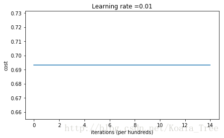
On the train set:
Accuracy: 0.5
On the test set:
Accuracy: 0.5

The performance is really bad, and the cost does not really decrease, and the algorithm performs no better than random guessing. Why? Lets look at the details of the predictions and the decision boundary:

print ("predictions_train = " + str(predictions_train))
print ("predictions_test = " + str(predictions_test))

predictions_train = [[0 0 0 0 0 0 0 0 0 0 0 0 0 0 0 0 0 0 0 0 0 0 0 0 0 0 0 0 0 0 0 0 0 0 0 0 0
  0 0 0 0 0 0 0 0 0 0 0 0 0 0 0 0 0 0 0 0 0 0 0 0 0 0 0 0 0 0 0 0 0 0 0 0 0
  0 0 0 0 0 0 0 0 0 0 0 0 0 0 0 0 0 0 0 0 0 0 0 0 0 0 0 0 0 0 0 0 0 0 0 0 0
  0 0 0 0 0 0 0 0 0 0 0 0 0 0 0 0 0 0 0 0 0 0 0 0 0 0 0 0 0 0 0 0 0 0 0 0 0
  0 0 0 0 0 0 0 0 0 0 0 0 0 0 0 0 0 0 0 0 0 0 0 0 0 0 0 0 0 0 0 0 0 0 0 0 0
  0 0 0 0 0 0 0 0 0 0 0 0 0 0 0 0 0 0 0 0 0 0 0 0 0 0 0 0 0 0 0 0 0 0 0 0 0
  0 0 0 0 0 0 0 0 0 0 0 0 0 0 0 0 0 0 0 0 0 0 0 0 0 0 0 0 0 0 0 0 0 0 0 0 0
  0 0 0 0 0 0 0 0 0 0 0 0 0 0 0 0 0 0 0 0 0 0 0 0 0 0 0 0 0 0 0 0 0 0 0 0 0
  0 0 0 0]]
predictions_test = [[0 0 0 0 0 0 0 0 0 0 0 0 0 0 0 0 0 0 0 0 0 0 0 0 0 0 0 0 0 0 0 0 0 0 0 0 0
  0 0 0 0 0 0 0 0 0 0 0 0 0 0 0 0 0 0 0 0 0 0 0 0 0 0 0 0 0 0 0 0 0 0 0 0 0
  0 0 0 0 0 0 0 0 0 0 0 0 0 0 0 0 0 0 0 0 0 0 0 0 0 0]]

plt.title("Model with Zeros initialization")
axes = plt.gca()
axes.set_xlim([-1.5,1.5])
axes.set_ylim([-1.5,1.5])
plot_decision_boundary(lambda x: predict_dec(parameters, x.T), train_X, train_Y)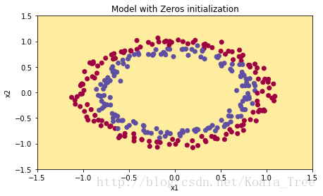

The model is predicting 0 for every example.

In general, initializing all the weights to zero results in the network failing to break symmetry. This means that every neuron in each layer will learn the same thing, and you might as well be training a neural network with $n^{[l]}=1$ for every layer, and the network is no more powerful than a linear classifier such as logistic regression.

What you should remember:
- The weights $W^{[l]}$ should be initialized randomly to break symmetry.
- It is however okay to initialize the biases $b^{[l]}$ to zeros. Symmetry is still broken so long as $W^{[l]}$ is initialized randomly.

3 - Random initialization

To break symmetry, lets intialize the weights randomly. Following random initialization, each neuron can then proceed to learn a different function of its inputs. In this exercise, you will see what happens if the weights are intialized randomly, but to very large values.

Exercise: Implement the following function to initialize your weights to large random values (scaled by *10) and your biases to zeros. Use np.random.randn(..,..) * 10 for weights and np.zeros((.., ..)) for biases. We are using a fixed np.random.seed(..) to make sure your “random” weights match ours, so don’t worry if running several times your code gives you always the same initial values for the parameters.

# GRADED FUNCTION: initialize_parameters_random

def initialize_parameters_random(layers_dims):
    """
    Arguments:
    layer_dims -- python array (list) containing the size of each layer.

    Returns:
    parameters -- python dictionary containing your parameters "W1", "b1", ..., "WL", "bL":
                    W1 -- weight matrix of shape (layers_dims[1], layers_dims[0])
                    b1 -- bias vector of shape (layers_dims[1], 1)
                    ...
                    WL -- weight matrix of shape (layers_dims[L], layers_dims[L-1])
                    bL -- bias vector of shape (layers_dims[L], 1)
    """

    np.random.seed(3)               # This seed makes sure your "random" numbers will be the as ours
    parameters = {}
    L = len(layers_dims)            # integer representing the number of layers

    for l in range(1, L):
        ### START CODE HERE ### (≈ 2 lines of code)
        parameters['W' + str(l)] = np.random.randn(layers_dims[l],layers_dims[l-1])*10
        parameters['b' + str(l)] = np.zeros((layers_dims[l],1))
        ### END CODE HERE ###

    return parameters

parameters = initialize_parameters_random([3, 2, 1])
print("W1 = " + str(parameters["W1"]))
print("b1 = " + str(parameters["b1"]))
print("W2 = " + str(parameters["W2"]))
print("b2 = " + str(parameters["b2"]))

W1 = [[ 17.88628473   4.36509851   0.96497468]
 [-18.63492703  -2.77388203  -3.54758979]]
b1 = [[ 0.]
 [ 0.]]
W2 = [[-0.82741481 -6.27000677]]
b2 = [[ 0.]]

Run the following code to train your model on 15,000 iterations using random initialization.

parameters = model(train_X, train_Y, initialization = "random")
print ("On the train set:")
predictions_train = predict(train_X, train_Y, parameters)
print ("On the test set:")
predictions_test = predict(test_X, test_Y, parameters)

Cost after iteration 0: inf
Cost after iteration 1000: 0.6237287551108738
Cost after iteration 2000: 0.5981106708339466
Cost after iteration 3000: 0.5638353726276827
Cost after iteration 4000: 0.550152614449184
Cost after iteration 5000: 0.5444235275228304
Cost after iteration 6000: 0.5374184054630083
Cost after iteration 7000: 0.47357131493578297
Cost after iteration 8000: 0.39775634899580387
Cost after iteration 9000: 0.3934632865981078
Cost after iteration 10000: 0.39202525076484457
Cost after iteration 11000: 0.38921493051297673
Cost after iteration 12000: 0.38614221789840486
Cost after iteration 13000: 0.38497849983013926
Cost after iteration 14000: 0.38278397192120406

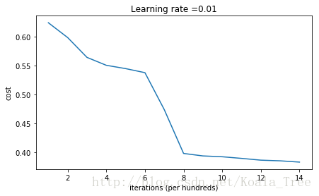
On the train set:
Accuracy: 0.83
On the test set:
Accuracy: 0.86

If you see “inf” as the cost after the iteration 0, this is because of numerical roundoff; a more numerically sophisticated implementation would fix this. But this isn’t worth worrying about for our purposes.

Anyway, it looks like you have broken symmetry, and this gives better results. than before. The model is no longer outputting all 0s.

print (predictions_train)
print (predictions_test)

[[1 0 1 1 0 0 1 1 1 1 1 0 1 0 0 1 0 1 1 0 0 0 1 0 1 1 1 1 1 1 0 1 1 0 0 1 1
  1 1 1 1 1 1 0 1 1 1 1 0 1 0 1 1 1 1 0 0 1 1 1 1 0 1 1 0 1 0 1 1 1 1 0 0 0
  0 0 1 0 1 0 1 1 1 0 0 1 1 1 1 1 1 0 0 1 1 1 0 1 1 0 1 0 1 1 0 1 1 0 1 0 1
  1 0 0 1 0 0 1 1 0 1 1 1 0 1 0 0 1 0 1 1 1 1 1 1 1 0 1 1 0 0 1 1 0 0 0 1 0
  1 0 1 0 1 1 1 0 0 1 1 1 1 0 1 1 0 1 0 1 1 0 1 0 1 1 1 1 0 1 1 1 1 0 1 0 1
  0 1 1 1 1 0 1 1 0 1 1 0 1 1 0 1 0 1 1 1 0 1 1 1 0 1 0 1 0 0 1 0 1 1 0 1 1
  0 1 1 0 1 1 1 0 1 1 1 1 0 1 0 0 1 1 0 1 1 1 0 0 0 1 1 0 1 1 1 1 0 1 1 0 1
  1 1 0 0 1 0 0 0 1 0 0 0 1 1 1 1 0 0 0 0 1 1 1 1 0 0 1 1 1 1 1 1 1 0 0 0 1
  1 1 1 0]]
[[1 1 1 1 0 1 0 1 1 0 1 1 1 0 0 0 0 1 0 1 0 0 1 0 1 0 1 1 1 1 1 0 0 0 0 1 0
  1 1 0 0 1 1 1 1 1 0 1 1 1 0 1 0 1 1 0 1 0 1 0 1 1 1 1 1 1 1 1 1 0 1 0 1 1
  1 1 1 0 1 0 0 1 0 0 0 1 1 0 1 1 0 0 0 1 1 0 1 1 0 0]]

plt.title("Model with large random initialization")
axes = plt.gca()
axes.set_xlim([-1.5,1.5])
axes.set_ylim([-1.5,1.5])
plot_decision_boundary(lambda x: predict_dec(parameters, x.T), train_X, train_Y)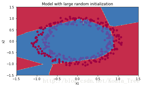

Observations:
- The cost starts very high. This is because with large random-valued weights, the last activation (sigmoid) outputs results that are very close to 0 or 1 for some examples, and when it gets that example wrong it incurs a very high loss for that example. Indeed, when $\log(a^{[3]}) = \log(0)$ , the loss goes to infinity.
- Poor initialization can lead to vanishing/exploding gradients, which also slows down the optimization algorithm.
- If you train this network longer you will see better results, but initializing with overly large random numbers slows down the optimization.

In summary:
- Initializing weights to very large random values does not work well.
- Hopefully intializing with small random values does better. The important question is: how small should be these random values be? Lets find out in the next part!

4 - He initialization

Finally, try “He Initialization”; this is named for the first author of He et al., 2015. (If you have heard of “Xavier initialization”, this is similar except Xavier initialization uses a scaling factor for the weights $W^{[l]}$ of sqrt(1./layers_dims[l-1]) where He initialization would use sqrt(2./layers_dims[l-1]).)

Exercise: Implement the following function to initialize your parameters with He initialization.

Hint: This function is similar to the previous initialize_parameters_random(...). The only difference is that instead of multiplying np.random.randn(..,..) by 10, you will multiply it by $\sqrt{\frac{2}{\text{dimension of the previous layer}}}$ , which is what He initialization recommends for layers with a ReLU activation.

# GRADED FUNCTION: initialize_parameters_he

def initialize_parameters_he(layers_dims):
    """
    Arguments:
    layer_dims -- python array (list) containing the size of each layer.

    Returns:
    parameters -- python dictionary containing your parameters "W1", "b1", ..., "WL", "bL":
                    W1 -- weight matrix of shape (layers_dims[1], layers_dims[0])
                    b1 -- bias vector of shape (layers_dims[1], 1)
                    ...
                    WL -- weight matrix of shape (layers_dims[L], layers_dims[L-1])
                    bL -- bias vector of shape (layers_dims[L], 1)
    """

    np.random.seed(3)
    parameters = {}
    L = len(layers_dims) - 1 # integer representing the number of layers

    for l in range(1, L + 1):
        ### START CODE HERE ### (≈ 2 lines of code)
        parameters['W' + str(l)] = np.random.randn(layers_dims[l],layers_dims[l-1])*np.sqrt(2./layers_dims[l-1])
        parameters['b' + str(l)] = np.zeros((layers_dims[l],1))
        ### END CODE HERE ###

    return parameters

parameters = initialize_parameters_he([2, 4, 1])
print("W1 = " + str(parameters["W1"]))
print("b1 = " + str(parameters["b1"]))
print("W2 = " + str(parameters["W2"]))
print("b2 = " + str(parameters["b2"]))

W1 = [[ 1.78862847  0.43650985]
 [ 0.09649747 -1.8634927 ]
 [-0.2773882  -0.35475898]
 [-0.08274148 -0.62700068]]
b1 = [[ 0.]
 [ 0.]
 [ 0.]
 [ 0.]]
W2 = [[-0.03098412 -0.33744411 -0.92904268  0.62552248]]
b2 = [[ 0.]]

Run the following code to train your model on 15,000 iterations using He initialization.

parameters = model(train_X, train_Y, initialization = "he")
print ("On the train set:")
predictions_train = predict(train_X, train_Y, parameters)
print ("On the test set:")
predictions_test = predict(test_X, test_Y, parameters)

Cost after iteration 0: 0.8830537463419761
Cost after iteration 1000: 0.6879825919728063
Cost after iteration 2000: 0.6751286264523371
Cost after iteration 3000: 0.6526117768893807
Cost after iteration 4000: 0.6082958970572938
Cost after iteration 5000: 0.5304944491717495
Cost after iteration 6000: 0.4138645817071794
Cost after iteration 7000: 0.3117803464844441
Cost after iteration 8000: 0.23696215330322562
Cost after iteration 9000: 0.18597287209206836
Cost after iteration 10000: 0.1501555628037182
Cost after iteration 11000: 0.12325079292273548
Cost after iteration 12000: 0.09917746546525937
Cost after iteration 13000: 0.0845705595402428
Cost after iteration 14000: 0.07357895962677366

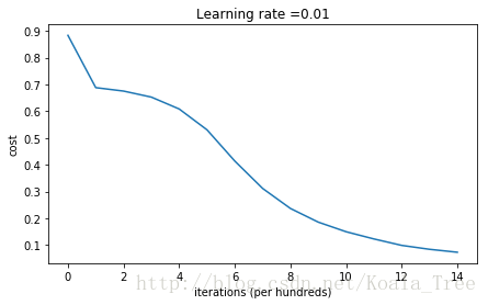
On the train set:
Accuracy: 0.993333333333
On the test set:
Accuracy: 0.96

plt.title("Model with He initialization")
axes = plt.gca()
axes.set_xlim([-1.5,1.5])
axes.set_ylim([-1.5,1.5])
plot_decision_boundary(lambda x: predict_dec(parameters, x.T), train_X, train_Y)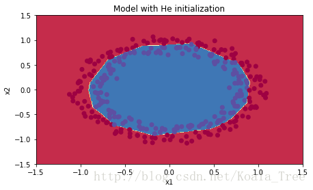

Observations:
- The model with He initialization separates the blue and the red dots very well in a small number of iterations.

5 - Conclusions

You have seen three different types of initializations. For the same number of iterations and same hyperparameters the comparison is:

Model	Train accuracy	Problem/Comment
3-layer NN with zeros initialization	50%	fails to break symmetry
3-layer NN with large random initialization	83%	too large weights
3-layer NN with He initialization	99%	recommended method

What you should remember from this notebook:
- Different initializations lead to different results
- Random initialization is used to break symmetry and make sure different hidden units can learn different things
- Don’t intialize to values that are too large
- He initialization works well for networks with ReLU activations.

Part 2：Regularization

Let’s first import the packages you are going to use.

# import packages
import numpy as np
import matplotlib.pyplot as plt
from reg_utils import sigmoid, relu, plot_decision_boundary, initialize_parameters, load_2D_dataset, predict_dec
from reg_utils import compute_cost, predict, forward_propagation, backward_propagation, update_parameters
import sklearn
import sklearn.datasets
import scipy.io
from testCases import *

%matplotlib inline
plt.rcParams['figure.figsize'] = (7.0, 4.0) # set default size of plots
plt.rcParams['image.interpolation'] = 'nearest'
plt.rcParams['image.cmap'] = 'gray'

There are some function iported：

def initialize_parameters(layer_dims):
    """
    Arguments:
    layer_dims -- python array (list) containing the dimensions of each layer in our network

    Returns:
    parameters -- python dictionary containing your parameters "W1", "b1", ..., "WL", "bL":
                    W1 -- weight matrix of shape (layer_dims[l], layer_dims[l-1])
                    b1 -- bias vector of shape (layer_dims[l], 1)
                    Wl -- weight matrix of shape (layer_dims[l-1], layer_dims[l])
                    bl -- bias vector of shape (1, layer_dims[l])

    Tips:
    - For example: the layer_dims for the "Planar Data classification model" would have been [2,2,1]. 
    This means W1's shape was (2,2), b1 was (1,2), W2 was (2,1) and b2 was (1,1). Now you have to generalize it!
    - In the for loop, use parameters['W' + str(l)] to access Wl, where l is the iterative integer.
    """

    np.random.seed(3)
    parameters = {}
    L = len(layer_dims) # number of layers in the network

    for l in range(1, L):
        parameters['W' + str(l)] = np.random.randn(layer_dims[l], layer_dims[l-1]) / np.sqrt(layer_dims[l-1])
        parameters['b' + str(l)] = np.zeros((layer_dims[l], 1))

        assert(parameters['W' + str(l)].shape == layer_dims[l], layer_dims[l-1])
        assert(parameters['W' + str(l)].shape == layer_dims[l], 1)


    return parameters


def compute_cost(a3, Y):
    """
    Implement the cost function

    Arguments:
    a3 -- post-activation, output of forward propagation
    Y -- "true" labels vector, same shape as a3

    Returns:
    cost - value of the cost function
    """
    m = Y.shape[1]

    logprobs = np.multiply(-np.log(a3),Y) + np.multiply(-np.log(1 - a3), 1 - Y)
    cost = 1./m * np.nansum(logprobs)

    return cost


def load_2D_dataset():
    data = scipy.io.loadmat('datasets/data.mat')
    train_X = data['X'].T
    train_Y = data['y'].T
    test_X = data['Xval'].T
    test_Y = data['yval'].T

    plt.scatter(train_X[0, :], train_X[1, :], c=train_Y, s=40, cmap=plt.cm.Spectral);

    return train_X, train_Y, test_X, test_Y

The data set in load_2D_dataset() ,you can get it in the address : http://pan.baidu.com/s/1sl4YzfB . If the link is invalid , please leave your message in the message area.

Problem Statement: You have just been hired as an AI expert by the French Football Corporation. They would like you to recommend positions where France’s goal keeper should kick the ball so that the French team’s players can then hit it with their head.

Figure 1 : Football field
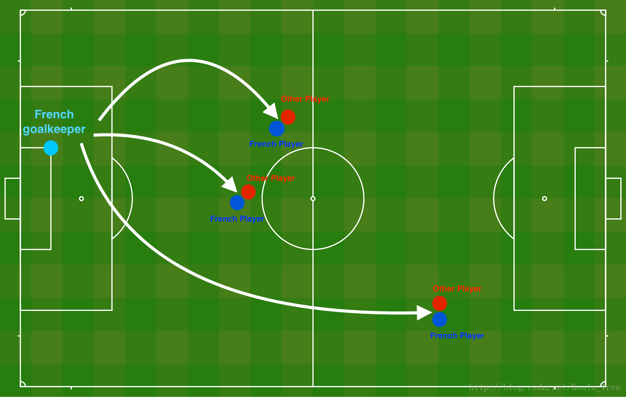
The goal keeper kicks the ball in the air, the players of each team are fighting to hit the ball with their head

They give you the following 2D dataset from France’s past 10 games.

train_X, train_Y, test_X, test_Y = load_2D_dataset()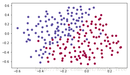

Each dot corresponds to a position on the football field where a football player has hit the ball with his/her head after the French goal keeper has shot the ball from the left side of the football field.
- If the dot is blue, it means the French player managed to hit the ball with his/her head
- If the dot is red, it means the other team’s player hit the ball with their head

Your goal: Use a deep learning model to find the positions on the field where the goalkeeper should kick the ball.

Analysis of the dataset: This dataset is a little noisy, but it looks like a diagonal line separating the upper left half (blue) from the lower right half (red) would work well.

You will first try a non-regularized model. Then you’ll learn how to regularize it and decide which model you will choose to solve the French Football Corporation’s problem.

1 - Non-regularized model

You will use the following neural network (already implemented for you below). This model can be used:
- in regularization mode – by setting the lambd input to a non-zero value. We use “lambd” instead of “lambda” because “lambda” is a reserved keyword in Python.
- in dropout mode – by setting the keep_prob to a value less than one

You will first try the model without any regularization. Then, you will implement:
- L2 regularization – functions: “compute_cost_with_regularization()” and “backward_propagation_with_regularization()”
- Dropout – functions: “forward_propagation_with_dropout()” and “backward_propagation_with_dropout()”

In each part, you will run this model with the correct inputs so that it calls the functions you’ve implemented. Take a look at the code below to familiarize yourself with the model.

def model(X, Y, learning_rate = 0.3, num_iterations = 30000, print_cost = True, lambd = 0, keep_prob = 1):
    """
    Implements a three-layer neural network: LINEAR->RELU->LINEAR->RELU->LINEAR->SIGMOID.

    Arguments:
    X -- input data, of shape (input size, number of examples)
    Y -- true "label" vector (1 for blue dot / 0 for red dot), of shape (output size, number of examples)
    learning_rate -- learning rate of the optimization
    num_iterations -- number of iterations of the optimization loop
    print_cost -- If True, print the cost every 10000 iterations
    lambd -- regularization hyperparameter, scalar
    keep_prob - probability of keeping a neuron active during drop-out, scalar.

    Returns:
    parameters -- parameters learned by the model. They can then be used to predict.
    """

    grads = {}
    costs = []                            # to keep track of the cost
    m = X.shape[1]                        # number of examples
    layers_dims = [X.shape[0], 20, 3, 1]

    # Initialize parameters dictionary.
    parameters = initialize_parameters(layers_dims)

    # Loop (gradient descent)

    for i in range(0, num_iterations):

        # Forward propagation: LINEAR -> RELU -> LINEAR -> RELU -> LINEAR -> SIGMOID.
        if keep_prob == 1:
            a3, cache = forward_propagation(X, parameters)
        elif keep_prob < 1:
            a3, cache = forward_propagation_with_dropout(X, parameters, keep_prob)

        # Cost function
        if lambd == 0:
            cost = compute_cost(a3, Y)
        else:
            cost = compute_cost_with_regularization(a3, Y, parameters, lambd)

        # Backward propagation.
        assert(lambd==0 or keep_prob==1)    # it is possible to use both L2 regularization and dropout, 
                                            # but this assignment will only explore one at a time
        if lambd == 0 and keep_prob == 1:
            grads = backward_propagation(X, Y, cache)
        elif lambd != 0:
            grads = backward_propagation_with_regularization(X, Y, cache, lambd)
        elif keep_prob < 1:
            grads = backward_propagation_with_dropout(X, Y, cache, keep_prob)

        # Update parameters.
        parameters = update_parameters(parameters, grads, learning_rate)

        # Print the loss every 10000 iterations
        if print_cost and i % 10000 == 0:
            print("Cost after iteration {}: {}".format(i, cost))
        if print_cost and i % 1000 == 0:
            costs.append(cost)

    # plot the cost
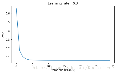
    plt.plot(costs)
    plt.ylabel('cost')
    plt.xlabel('iterations (x1,000)')
    plt.title("Learning rate =" + str(learning_rate))
    plt.show()

    return parameters

Let’s train the model without any regularization, and observe the accuracy on the train/test sets.

parameters = model(train_X, train_Y)
print ("On the training set:")
predictions_train = predict(train_X, train_Y, parameters)
print ("On the test set:")
predictions_test = predict(test_X, test_Y, parameters)

Cost after iteration 0: 0.6557412523481002
Cost after iteration 10000: 0.16329987525724216
Cost after iteration 20000: 0.13851642423255986

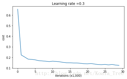
On the training set:
Accuracy: 0.947867298578
On the test set:
Accuracy: 0.915

The train accuracy is 94.8% while the test accuracy is 91.5%. This is the baseline model (you will observe the impact of regularization on this model). Run the following code to plot the decision boundary of your model.

plt.title("Model without regularization")
axes = plt.gca()
axes.set_xlim([-0.75,0.40])
axes.set_ylim([-0.75,0.65])
plot_decision_boundary(lambda x: predict_dec(parameters, x.T), train_X, train_Y)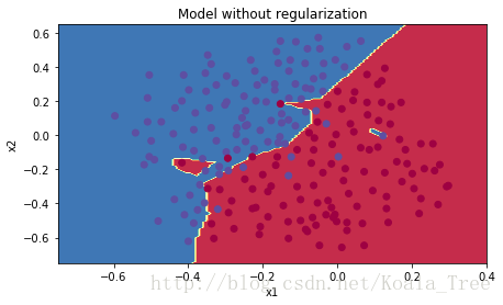

The non-regularized model is obviously overfitting the training set. It is fitting the noisy points! Lets now look at two techniques to reduce overfitting.

2 - L2 Regularization

The standard way to avoid overfitting is called L2 regularization. It consists of appropriately modifying your cost function, from:

J = - 1 m \sum i = 1 m (y (i) log (a [L] (i)) + (1 - y (i)) log (1 - a [L] (i))) (1)

$J = -\frac{1}{m} \sum\limits_{i = 1}^{m} \large{(}\small y^{(i)}\log\left(a^{[L](i)}\right) + (1-y^{(i)})\log\left(1- a^{[L](i)}\right) \large{)} \tag{1}$
To:

J r e g u l a r i z e d = - 1 m \sum i = 1 m (y (i) log (a [L] (i)) + (1 - y (i)) log (1 - a [L] (i)))                                                                cross-entropy cost + 1 m λ 2 \sum l \sum k \sum j W [l] 2 k, j                          L2 regularization cost (2)

$J_{regularized} = \small \underbrace{-\frac{1}{m} \sum\limits_{i = 1}^{m} \large{(}\small y^{(i)}\log\left(a^{[L](i)}\right) + (1-y^{(i)})\log\left(1- a^{[L](i)}\right) \large{)} }_\text{cross-entropy cost} + \underbrace{\frac{1}{m} \frac{\lambda}{2} \sum\limits_l\sum\limits_k\sum\limits_j W_{k,j}^{[l]2} }_\text{L2 regularization cost} \tag{2}$

Let’s modify your cost and observe the consequences.

Exercise: Implement compute_cost_with_regularization() which computes the cost given by formula (2). To calculate $\sum\limits_k\sum\limits_j W_{k,j}^{[l]2}$ , use :

np.sum(np.square(Wl))

Note that you have to do this for $W^{[1]}$ , $W^{[2]}$ and $W^{[3]}$ , then sum the three terms and multiply by $\frac{1}{m} \frac{\lambda}{2}$ .

# GRADED FUNCTION: compute_cost_with_regularization

def compute_cost_with_regularization(A3, Y, parameters, lambd):
    """
    Implement the cost function with L2 regularization. See formula (2) above.

    Arguments:
    A3 -- post-activation, output of forward propagation, of shape (output size, number of examples)
    Y -- "true" labels vector, of shape (output size, number of examples)
    parameters -- python dictionary containing parameters of the model

    Returns:
    cost - value of the regularized loss function (formula (2))
    """
    m = Y.shape[1]
    W1 = parameters["W1"]
    W2 = parameters["W2"]
    W3 = parameters["W3"]

    cross_entropy_cost = compute_cost(A3, Y) # This gives you the cross-entropy part of the cost

    ### START CODE HERE ### (approx. 1 line)
    L2_regularization_cost = (1./m*lambd/2)*(np.sum(np.square(W1)) + np.sum(np.square(W2)) + np.sum(np.square(W3)))
    ### END CODER HERE ###

    cost = cross_entropy_cost + L2_regularization_cost

    return cost

A3, Y_assess, parameters = compute_cost_with_regularization_test_case()

print("cost = " + str(compute_cost_with_regularization(A3, Y_assess, parameters, lambd = 0.1)))

cost = 1.78648594516

Of course, because you changed the cost, you have to change backward propagation as well! All the gradients have to be computed with respect to this new cost.

Exercise: Implement the changes needed in backward propagation to take into account regularization. The changes only concern dW1, dW2 and dW3. For each, you have to add the regularization term’s gradient ( $\frac{d}{dW} ( \frac{1}{2}\frac{\lambda}{m} W^2) = \frac{\lambda}{m} W$ ).

# GRADED FUNCTION: backward_propagation_with_regularization

def backward_propagation_with_regularization(X, Y, cache, lambd):
    """
    Implements the backward propagation of our baseline model to which we added an L2 regularization.

    Arguments:
    X -- input dataset, of shape (input size, number of examples)
    Y -- "true" labels vector, of shape (output size, number of examples)
    cache -- cache output from forward_propagation()
    lambd -- regularization hyperparameter, scalar

    Returns:
    gradients -- A dictionary with the gradients with respect to each parameter, activation and pre-activation variables
    """

    m = X.shape[1]
    (Z1, A1, W1, b1, Z2, A2, W2, b2, Z3, A3, W3, b3) = cache

    dZ3 = A3 - Y

    ### START CODE HERE ### (approx. 1 line)
    dW3 = 1./m * np.dot(dZ3, A2.T) + lambd/m * W3
    ### END CODE HERE ###
    db3 = 1./m * np.sum(dZ3, axis=1, keepdims = True)

    dA2 = np.dot(W3.T, dZ3)
    dZ2 = np.multiply(dA2, np.int64(A2 > 0))
    ### START CODE HERE ### (approx. 1 line)
    dW2 = 1./m * np.dot(dZ2, A1.T) + lambd/m * W2
    ### END CODE HERE ###
    db2 = 1./m * np.sum(dZ2, axis=1, keepdims = True)

    dA1 = np.dot(W2.T, dZ2)
    dZ1 = np.multiply(dA1, np.int64(A1 > 0))
    ### START CODE HERE ### (approx. 1 line)
    dW1 = 1./m * np.dot(dZ1, X.T) + lambd/m * W1
    ### END CODE HERE ###
    db1 = 1./m * np.sum(dZ1, axis=1, keepdims = True)

    gradients = {"dZ3": dZ3, "dW3": dW3, "db3": db3,"dA2": dA2,
                 "dZ2": dZ2, "dW2": dW2, "db2": db2, "dA1": dA1, 
                 "dZ1": dZ1, "dW1": dW1, "db1": db1}

    return gradients

X_assess, Y_assess, cache = backward_propagation_with_regularization_test_case()

grads = backward_propagation_with_regularization(X_assess, Y_assess, cache, lambd = 0.7)
print ("dW1 = "+ str(grads["dW1"]))
print ("dW2 = "+ str(grads["dW2"]))
print ("dW3 = "+ str(grads["dW3"]))

dW1 = [[-0.25604646  0.12298827 -0.28297129]
 [-0.17706303  0.34536094 -0.4410571 ]]
dW2 = [[ 0.79276486  0.85133918]
 [-0.0957219  -0.01720463]
 [-0.13100772 -0.03750433]]
dW3 = [[-1.77691347 -0.11832879 -0.09397446]]

Let’s now run the model with L2 regularization $(\lambda = 0.7)$ . The model() function will call:
- compute_cost_with_regularization instead of compute_cost
- backward_propagation_with_regularization instead of backward_propagation

parameters = model(train_X, train_Y, lambd = 0.7)
print ("On the train set:")
predictions_train = predict(train_X, train_Y, parameters)
print ("On the test set:")
predictions_test = predict(test_X, test_Y, parameters)

Cost after iteration 0: 0.6974484493131264
Cost after iteration 10000: 0.2684918873282239
Cost after iteration 20000: 0.2680916337127301

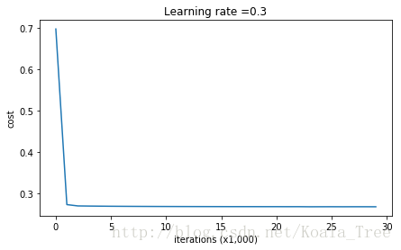
On the train set:
Accuracy: 0.938388625592
On the test set:
Accuracy: 0.93

Congrats, the test set accuracy increased to 93%. You have saved the French football team!

You are not overfitting the training data anymore. Let’s plot the decision boundary.

plt.title("Model with L2-regularization")
axes = plt.gca()
axes.set_xlim([-0.75,0.40])
axes.set_ylim([-0.75,0.65])
plot_decision_boundary(lambda x: predict_dec(parameters, x.T), train_X, train_Y)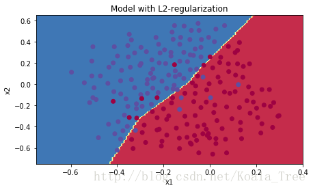

Observations:
- The value of $\lambda$ is a hyperparameter that you can tune using a dev set.
- L2 regularization makes your decision boundary smoother. If $\lambda$ is too large, it is also possible to “oversmooth”, resulting in a model with high bias.

What is L2-regularization actually doing?:

L2-regularization relies on the assumption that a model with small weights is simpler than a model with large weights. Thus, by penalizing the square values of the weights in the cost function you drive all the weights to smaller values. It becomes too costly for the cost to have large weights! This leads to a smoother model in which the output changes more slowly as the input changes.

What you should remember – the implications of L2-regularization on:
- The cost computation:
- A regularization term is added to the cost
- The backpropagation function:
- There are extra terms in the gradients with respect to weight matrices
- Weights end up smaller (“weight decay”):
- Weights are pushed to smaller values.

3 - Dropout

Finally, dropout is a widely used regularization technique that is specific to deep learning.
It randomly shuts down some neurons in each iteration.

When you shut some neurons down, you actually modify your model. The idea behind drop-out is that at each iteration, you train a different model that uses only a subset of your neurons. With dropout, your neurons thus become less sensitive to the activation of one other specific neuron, because that other neuron might be shut down at any time.

3.1 - Forward propagation with dropout

Exercise: Implement the forward propagation with dropout. You are using a 3 layer neural network, and will add dropout to the first and second hidden layers. We will not apply dropout to the input layer or output layer.

Instructions:
You would like to shut down some neurons in the first and second layers. To do that, you are going to carry out 4 Steps:
1. In lecture, we dicussed creating a variable $d^{[1]}$ with the same shape as $a^{[1]}$ using np.random.rand() to randomly get numbers between 0 and 1. Here, you will use a vectorized implementation, so create a random matrix $D^{[1]} = [d^{[1](1)} d^{[1](2)} ... d^{[1](m)}]$ of the same dimension as $A^{[1]}$ .
2. Set each entry of $D^{[1]}$ to be 0 with probability (1-keep_prob) or 1 with probability (keep_prob), by thresholding values in $D^{[1]}$ appropriately. Hint: to set all the entries of a matrix X to 0 (if entry is less than 0.5) or 1 (if entry is more than 0.5) you would do: X = (X < 0.5). Note that 0 and 1 are respectively equivalent to False and True.
3. Set $A^{[1]}$ to $A^{[1]} * D^{[1]}$ . (You are shutting down some neurons). You can think of $D^{[1]}$ as a mask, so that when it is multiplied with another matrix, it shuts down some of the values.
4. Divide $A^{[1]}$ by keep_prob. By doing this you are assuring that the result of the cost will still have the same expected value as without drop-out. (This technique is also called inverted dropout.)

# GRADED FUNCTION: forward_propagation_with_dropout

def forward_propagation_with_dropout(X, parameters, keep_prob = 0.5):
    """
    Implements the forward propagation: LINEAR -> RELU + DROPOUT -> LINEAR -> RELU + DROPOUT -> LINEAR -> SIGMOID.

    Arguments:
    X -- input dataset, of shape (2, number of examples)
    parameters -- python dictionary containing your parameters "W1", "b1", "W2", "b2", "W3", "b3":
                    W1 -- weight matrix of shape (20, 2)
                    b1 -- bias vector of shape (20, 1)
                    W2 -- weight matrix of shape (3, 20)
                    b2 -- bias vector of shape (3, 1)
                    W3 -- weight matrix of shape (1, 3)
                    b3 -- bias vector of shape (1, 1)
    keep_prob - probability of keeping a neuron active during drop-out, scalar

    Returns:
    A3 -- last activation value, output of the forward propagation, of shape (1,1)
    cache -- tuple, information stored for computing the backward propagation
    """

    np.random.seed(1)

    # retrieve parameters
    W1 = parameters["W1"]
    b1 = parameters["b1"]
    W2 = parameters["W2"]
    b2 = parameters["b2"]
    W3 = parameters["W3"]
    b3 = parameters["b3"]

    # LINEAR -> RELU -> LINEAR -> RELU -> LINEAR -> SIGMOID
    Z1 = np.dot(W1, X) + b1
    A1 = relu(Z1)
    ### START CODE HERE ### (approx. 4 lines)         # Steps 1-4 below correspond to the Steps 1-4 described above. 
    D1 = np.random.rand(A1.shape[0],A1.shape[1])                                         # Step 1: initialize matrix D1 = np.random.rand(..., ...)
    D1 = D1 < keep_prob                                      # Step 2: convert entries of D1 to 0 or 1 (using keep_prob as the threshold)
    A1 = A1 * D1                                         # Step 3: shut down some neurons of A1
    A1 = A1 / keep_prob                                        # Step 4: scale the value of neurons that haven't been shut down
    ### END CODE HERE ###
    Z2 = np.dot(W2, A1) + b2
    A2 = relu(Z2)
    ### START CODE HERE ### (approx. 4 lines)
    D2 = np.random.rand(A2.shape[0],A2.shape[1])                                         # Step 1: initialize matrix D2 = np.random.rand(..., ...)
    D2 = D2 < keep_prob                                         # Step 2: convert entries of D2 to 0 or 1 (using keep_prob as the threshold)
    A2 = A2 * D2                                         # Step 3: shut down some neurons of A2
    A2 = A2 / keep_prob                                      # Step 4: scale the value of neurons that haven't been shut down
    ### END CODE HERE ###
    Z3 = np.dot(W3, A2) + b3
    A3 = sigmoid(Z3)

    cache = (Z1, D1, A1, W1, b1, Z2, D2, A2, W2, b2, Z3, A3, W3, b3)

    return A3, cache

X_assess, parameters = forward_propagation_with_dropout_test_case()

A3, cache = forward_propagation_with_dropout(X_assess, parameters, keep_prob = 0.7)
print ("A3 = " + str(A3))

A3 = [[ 0.36974721  0.00305176  0.04565099  0.49683389  0.36974721]]

3.2 - Backward propagation with dropout

Exercise: Implement the backward propagation with dropout. As before, you are training a 3 layer network. Add dropout to the first and second hidden layers, using the masks $D^{[1]}$ and $D^{[2]}$ stored in the cache.

Instruction:
Backpropagation with dropout is actually quite easy. You will have to carry out 2 Steps:
1. You had previously shut down some neurons during forward propagation, by applying a mask $D^{[1]}$ to A1. In backpropagation, you will have to shut down the same neurons, by reapplying the same mask $D^{[1]}$ to dA1.
2. During forward propagation, you had divided A1 by keep_prob. In backpropagation, you’ll therefore have to divide dA1 by keep_prob again (the calculus interpretation is that if $A^{[1]}$ is scaled by keep_prob, then its derivative $dA^{[1]}$ is also scaled by the same keep_prob).

# GRADED FUNCTION: backward_propagation_with_dropout

def backward_propagation_with_dropout(X, Y, cache, keep_prob):
    """
    Implements the backward propagation of our baseline model to which we added dropout.

    Arguments:
    X -- input dataset, of shape (2, number of examples)
    Y -- "true" labels vector, of shape (output size, number of examples)
    cache -- cache output from forward_propagation_with_dropout()
    keep_prob - probability of keeping a neuron active during drop-out, scalar

    Returns:
    gradients -- A dictionary with the gradients with respect to each parameter, activation and pre-activation variables
    """

    m = X.shape[1]
    (Z1, D1, A1, W1, b1, Z2, D2, A2, W2, b2, Z3, A3, W3, b3) = cache

    dZ3 = A3 - Y
    dW3 = 1./m * np.dot(dZ3, A2.T)
    db3 = 1./m * np.sum(dZ3, axis=1, keepdims = True)
    dA2 = np.dot(W3.T, dZ3)
    ### START CODE HERE ### (≈ 2 lines of code)
    dA2 = dA2 * D2              # Step 1: Apply mask D2 to shut down the same neurons as during the forward propagation
    dA2 = dA2 / keep_prob           # Step 2: Scale the value of neurons that haven't been shut down
    ### END CODE HERE ###
    dZ2 = np.multiply(dA2, np.int64(A2 > 0))
    dW2 = 1./m * np.dot(dZ2, A1.T)
    db2 = 1./m * np.sum(dZ2, axis=1, keepdims = True)

    dA1 = np.dot(W2.T, dZ2)
    ### START CODE HERE ### (≈ 2 lines of code)
    dA1 = dA1 * D1              # Step 1: Apply mask D1 to shut down the same neurons as during the forward propagation
    dA1 = dA1 / keep_prob             # Step 2: Scale the value of neurons that haven't been shut down
    ### END CODE HERE ###
    dZ1 = np.multiply(dA1, np.int64(A1 > 0))
    dW1 = 1./m * np.dot(dZ1, X.T)
    db1 = 1./m * np.sum(dZ1, axis=1, keepdims = True)

    gradients = {"dZ3": dZ3, "dW3": dW3, "db3": db3,"dA2": dA2,
                 "dZ2": dZ2, "dW2": dW2, "db2": db2, "dA1": dA1, 
                 "dZ1": dZ1, "dW1": dW1, "db1": db1}

    return gradients

X_assess, Y_assess, cache = backward_propagation_with_dropout_test_case()

gradients = backward_propagation_with_dropout(X_assess, Y_assess, cache, keep_prob = 0.8)

print ("dA1 = " + str(gradients["dA1"]))
print ("dA2 = " + str(gradients["dA2"]))

dA1 = [[ 0.36544439  0.         -0.00188233  0.         -0.17408748]
 [ 0.65515713  0.         -0.00337459  0.         -0.        ]]
dA2 = [[ 0.58180856  0.         -0.00299679  0.         -0.27715731]
 [ 0.          0.53159854 -0.          0.53159854 -0.34089673]
 [ 0.          0.         -0.00292733  0.         -0.        ]]

Let’s now run the model with dropout (keep_prob = 0.86). It means at every iteration you shut down each neurons of layer 1 and 2 with 24% probability. The function model() will now call:
- forward_propagation_with_dropout instead of forward_propagation.
- backward_propagation_with_dropout instead of backward_propagation.

parameters = model(train_X, train_Y, keep_prob = 0.86, learning_rate = 0.3)

print ("On the train set:")
predictions_train = predict(train_X, train_Y, parameters)
print ("On the test set:")
predictions_test = predict(test_X, test_Y, parameters)

Cost after iteration 0: 0.6543912405149825
Cost after iteration 10000: 0.06101698657490559
Cost after iteration 20000: 0.060582435798513114

On the train set:
Accuracy: 0.928909952607
On the test set:
Accuracy: 0.95

Dropout works great! The test accuracy has increased again (to 95%)! Your model is not overfitting the training set and does a great job on the test set. The French football team will be forever grateful to you!

Run the code below to plot the decision boundary.

plt.title("Model with dropout")
axes = plt.gca()
axes.set_xlim([-0.75,0.40])
axes.set_ylim([-0.75,0.65])
plot_decision_boundary(lambda x: predict_dec(parameters, x.T), train_X, train_Y)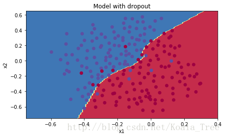

Note:
- A common mistake when using dropout is to use it both in training and testing. You should use dropout (randomly eliminate nodes) only in training.
- Deep learning frameworks like tensorflow, PaddlePaddle, keras or caffe come with a dropout layer implementation. Don’t stress - you will soon learn some of these frameworks.

What you should remember about dropout:
- Dropout is a regularization technique.
- You only use dropout during training. Don’t use dropout (randomly eliminate nodes) during test time.
- Apply dropout both during forward and backward propagation.
- During training time, divide each dropout layer by keep_prob to keep the same expected value for the activations. For example, if keep_prob is 0.5, then we will on average shut down half the nodes, so the output will be scaled by 0.5 since only the remaining half are contributing to the solution. Dividing by 0.5 is equivalent to multiplying by 2. Hence, the output now has the same expected value. You can check that this works even when keep_prob is other values than 0.5.

4 - Conclusions

Here are the results of our three models:

model	train accuracy	test accuracy
3-layer NN without regularization	95%	91.5%
3-layer NN with L2-regularization	94%	93%
3-layer NN with dropout	93%	95%

Note that regularization hurts training set performance! This is because it limits the ability of the network to overfit to the training set. But since it ultimately gives better test accuracy, it is helping your system.

Congratulations for finishing this assignment! And also for revolutionizing French football. :-)

What we want you to remember from this notebook:
- Regularization will help you reduce overfitting.
- Regularization will drive your weights to lower values.
- L2 regularization and Dropout are two very effective regularization techniques.

Part 3：Gradient Checking

First import the libs which you will need.

# Packages
import numpy as np
from testCases import *
from gc_utils import sigmoid, relu, dictionary_to_vector, vector_to_dictionary, gradients_to_vector

There are some function the program concerned：

def dictionary_to_vector(parameters):
    """
    Roll all our parameters dictionary into a single vector satisfying our specific required shape.
    """
    keys = []
    count = 0
    for key in ["W1", "b1", "W2", "b2", "W3", "b3"]:

        # flatten parameter
        new_vector = np.reshape(parameters[key], (-1,1))
        keys = keys + [key]*new_vector.shape[0]

        if count == 0:
            theta = new_vector
        else:
            theta = np.concatenate((theta, new_vector), axis=0)
        count = count + 1

    return theta, keys


def vector_to_dictionary(theta):
    """
    Unroll all our parameters dictionary from a single vector satisfying our specific required shape.
    """
    parameters = {}
    parameters["W1"] = theta[:20].reshape((5,4))
    parameters["b1"] = theta[20:25].reshape((5,1))
    parameters["W2"] = theta[25:40].reshape((3,5))
    parameters["b2"] = theta[40:43].reshape((3,1))
    parameters["W3"] = theta[43:46].reshape((1,3))
    parameters["b3"] = theta[46:47].reshape((1,1))

    return parameters


def gradients_to_vector(gradients):
    """
    Roll all our gradients dictionary into a single vector satisfying our specific required shape.
    """

    count = 0
    for key in ["dW1", "db1", "dW2", "db2", "dW3", "db3"]:
        # flatten parameter
        new_vector = np.reshape(gradients[key], (-1,1))

        if count == 0:
            theta = new_vector
        else:
            theta = np.concatenate((theta, new_vector), axis=0)
        count = count + 1

    return theta

1. How does gradient checking work?

Backpropagation computes the gradients $\frac{\partial J}{\partial \theta}$ , where $\theta$ denotes the parameters of the model. $J$ is computed using forward propagation and your loss function.

Because forward propagation is relatively easy to implement, you’re confident you got that right, and so you’re almost 100% sure that you’re computing the cost $J$ correctly. Thus, you can use your code for computing $J$ to verify the code for computing $\frac{\partial J}{\partial \theta}$ .

Let’s look back at the definition of a derivative (or gradient):

\partial J \partial θ = lim ε \to 0 J ( θ + ε ) - J ( θ - ε ) 2 ε (1)

$\frac{\partial J}{\partial \theta} = \lim_{\varepsilon \to 0} \frac{J(\theta + \varepsilon) - J(\theta - \varepsilon)}{2 \varepsilon} \tag{1}$

If you’re not familiar with the “ $\displaystyle \lim_{\varepsilon \to 0}$ ” notation, it’s just a way of saying “when $\varepsilon$ is really really small.”

We know the following:

$\frac{\partial J}{\partial \theta}$ is what you want to make sure you’re computing correctly.
You can compute $J(\theta + \varepsilon)$ and $J(\theta - \varepsilon)$ (in the case that $\theta$ is a real number), since you’re confident your implementation for $J$ is correct.

Lets use equation (1) and a small value for $\varepsilon$ to convince your CEO that your code for computing $\frac{\partial J}{\partial \theta}$ is correct!

2. 1-dimensional gradient checking

Consider a 1D linear function $J(\theta) = \theta x$ . The model contains only a single real-valued parameter $\theta$ , and takes $x$ as input.

You will implement code to compute $J(.)$ and its derivative $\frac{\partial J}{\partial \theta}$ . You will then use gradient checking to make sure your derivative computation for $J$ is correct.

Figure 1 : 1D linear model

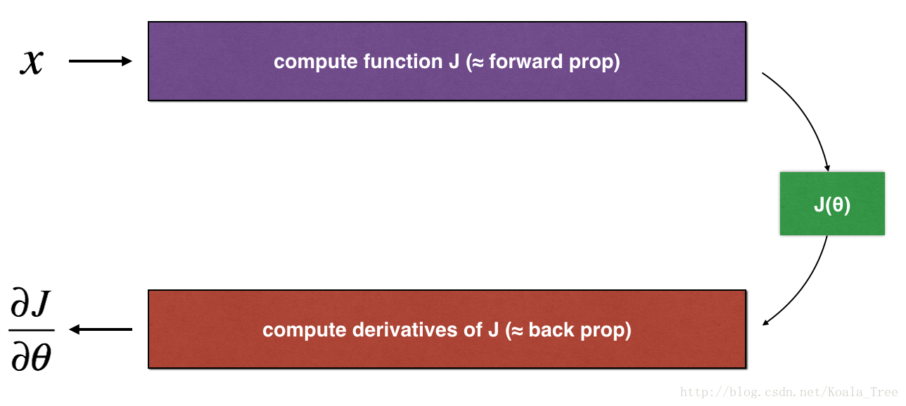
The diagram above shows the key computation steps: First start with $x$ , then evaluate the function $J(x)$ (“forward propagation”). Then compute the derivative $\frac{\partial J}{\partial \theta}$ (“backward propagation”).

Exercise: implement “forward propagation” and “backward propagation” for this simple function. I.e., compute both $J(.)$ (“forward propagation”) and its derivative with respect to $\theta$ (“backward propagation”), in two separate functions.

# GRADED FUNCTION: forward_propagation

def forward_propagation(x, theta):
    """
    Implement the linear forward propagation (compute J) presented in Figure 1 (J(theta) = theta * x)

    Arguments:
    x -- a real-valued input
    theta -- our parameter, a real number as well

    Returns:
    J -- the value of function J, computed using the formula J(theta) = theta * x
    """

    ### START CODE HERE ### (approx. 1 line)
    J = theta * x
    ### END CODE HERE ###

    return J

x, theta = 2, 4
J = forward_propagation(x, theta)
print ("J = " + str(J))

J = 8

Exercise: Now, implement the backward propagation step (derivative computation) of Figure 1. That is, compute the derivative of $J(\theta) = \theta x$ with respect to $\theta$ . To save you from doing the calculus, you should get $dtheta = \frac { \partial J }{ \partial \theta} = x$ .

# GRADED FUNCTION: backward_propagation

def backward_propagation(x, theta):
    """
    Computes the derivative of J with respect to theta (see Figure 1).

    Arguments:
    x -- a real-valued input
    theta -- our parameter, a real number as well

    Returns:
    dtheta -- the gradient of the cost with respect to theta
    """

    ### START CODE HERE ### (approx. 1 line)
    dtheta = x
    ### END CODE HERE ###

    return dtheta

x, theta = 2, 4
dtheta = backward_propagation(x, theta)
print ("dtheta = " + str(dtheta))

dtheta = 2

Exercise: To show that the backward_propagation() function is correctly computing the gradient $\frac{\partial J}{\partial \theta}$ , let’s implement gradient checking.

Instructions:
- First compute “gradapprox” using the formula above (1) and a small value of $\varepsilon$ . Here are the Steps to follow:
1. $\theta^{+} = \theta + \varepsilon$
2. $\theta^{-} = \theta - \varepsilon$
3. $J^{+} = J(\theta^{+})$
4. $J^{-} = J(\theta^{-})$
5. $gradapprox = \frac{J^{+} - J^{-}}{2 \varepsilon}$
- Then compute the gradient using backward propagation, and store the result in a variable “grad”
- Finally, compute the relative difference between “gradapprox” and the “grad” using the following formula:

d i f f e r e n c e = ∣ ∣ g r a d - g r a d a p p r o x ∣ ∣ 2 ∣ ∣ g r a d ∣ ∣ 2 + ∣ ∣ g r a d a p p r o x ∣ ∣ 2 (2)

$difference = \frac {\mid\mid grad - gradapprox \mid\mid_2}{\mid\mid grad \mid\mid_2 + \mid\mid gradapprox \mid\mid_2} \tag{2}$
You will need 3 Steps to compute this formula:
-1’. compute the numerator using np.linalg.norm(…)
- 2’. compute the denominator. You will need to call np.linalg.norm(…) twice.
- 3’. divide them.
- If this difference is small (say less than

10−7 10 − 7 $10^{-7}$ ), you can be quite confident that you have computed your gradient correctly. Otherwise, there may be a mistake in the gradient computation.

# GRADED FUNCTION: gradient_check

def gradient_check(x, theta, epsilon = 1e-7):
    """
    Implement the backward propagation presented in Figure 1.

    Arguments:
    x -- a real-valued input
    theta -- our parameter, a real number as well
    epsilon -- tiny shift to the input to compute approximated gradient with formula(1)

    Returns:
    difference -- difference (2) between the approximated gradient and the backward propagation gradient
    """

    # Compute gradapprox using left side of formula (1). epsilon is small enough, you don't need to worry about the limit.
    ### START CODE HERE ### (approx. 5 lines)
    thetaplus = theta + epsilon                               # Step 1
    thetaminus = theta - epsilon                              # Step 2
    J_plus = forward_propagation(x, thetaplus)                                  # Step 3
    J_minus = forward_propagation(x, thetaminus)                                 # Step 4
    gradapprox = (J_plus - J_minus) / (2 * epsilon)                              # Step 5
    ### END CODE HERE ###

    # Check if gradapprox is close enough to the output of backward_propagation()
    ### START CODE HERE ### (approx. 1 line)
    grad = backward_propagation(x, theta)
    ### END CODE HERE ###

    ### START CODE HERE ### (approx. 1 line)
    numerator = np.linalg.norm(grad - gradapprox)                               # Step 1'
    denominator = np.linalg.norm(grad) + np.linalg.norm(gradapprox)                            # Step 2'
    difference = numerator / denominator                              # Step 3'
    ### END CODE HERE ###

    if difference < 1e-7:
        print ("The gradient is correct!")
    else:
        print ("The gradient is wrong!")

    return difference

x, theta = 2, 4
difference = gradient_check(x, theta)
print("difference = " + str(difference))

The gradient is correct!
difference = 2.91933588329e-10

Congrats, the difference is smaller than the $10^{-7}$ threshold. So you can have high confidence that you’ve correctly computed the gradient in backward_propagation().

Now, in the more general case, your cost function $J$ has more than a single 1D input. When you are training a neural network, $\theta$ actually consists of multiple matrices $W^{[l]}$ and biases $b^{[l]}$ ! It is important to know how to do a gradient check with higher-dimensional inputs. Let’s do it!

3. N-dimensional gradient checking

The following figure describes the forward and backward propagation of your fraud detection model.

Figure 2 : deep neural network
LINEAR -> RELU -> LINEAR -> RELU -> LINEAR -> SIGMOID

Let’s look at your implementations for forward propagation and backward propagation.

def forward_propagation_n(X, Y, parameters):
    """
    Implements the forward propagation (and computes the cost) presented in Figure 3.

    Arguments:
    X -- training set for m examples
    Y -- labels for m examples 
    parameters -- python dictionary containing your parameters "W1", "b1", "W2", "b2", "W3", "b3":
                    W1 -- weight matrix of shape (5, 4)
                    b1 -- bias vector of shape (5, 1)
                    W2 -- weight matrix of shape (3, 5)
                    b2 -- bias vector of shape (3, 1)
                    W3 -- weight matrix of shape (1, 3)
                    b3 -- bias vector of shape (1, 1)

    Returns:
    cost -- the cost function (logistic cost for one example)
    """

    # retrieve parameters
    m = X.shape[1]
    W1 = parameters["W1"]
    b1 = parameters["b1"]
    W2 = parameters["W2"]
    b2 = parameters["b2"]
    W3 = parameters["W3"]
    b3 = parameters["b3"]

    # LINEAR -> RELU -> LINEAR -> RELU -> LINEAR -> SIGMOID
    Z1 = np.dot(W1, X) + b1
    A1 = relu(Z1)
    Z2 = np.dot(W2, A1) + b2
    A2 = relu(Z2)
    Z3 = np.dot(W3, A2) + b3
    A3 = sigmoid(Z3)

    # Cost
    logprobs = np.multiply(-np.log(A3),Y) + np.multiply(-np.log(1 - A3), 1 - Y)
    cost = 1./m * np.sum(logprobs)

    cache = (Z1, A1, W1, b1, Z2, A2, W2, b2, Z3, A3, W3, b3)

    return cost, cache

Now, run backward propagation.

def backward_propagation_n(X, Y, cache):
    """
    Implement the backward propagation presented in figure 2.

    Arguments:
    X -- input datapoint, of shape (input size, 1)
    Y -- true "label"
    cache -- cache output from forward_propagation_n()

    Returns:
    gradients -- A dictionary with the gradients of the cost with respect to each parameter, activation and pre-activation variables.
    """

    m = X.shape[1]
    (Z1, A1, W1, b1, Z2, A2, W2, b2, Z3, A3, W3, b3) = cache

    dZ3 = A3 - Y
    dW3 = 1./m * np.dot(dZ3, A2.T)
    db3 = 1./m * np.sum(dZ3, axis=1, keepdims = True)

    dA2 = np.dot(W3.T, dZ3)
    dZ2 = np.multiply(dA2, np.int64(A2 > 0))
    dW2 = 1./m * np.dot(dZ2, A1.T)
    db2 = 1./m * np.sum(dZ2, axis=1, keepdims = True)

    dA1 = np.dot(W2.T, dZ2)
    dZ1 = np.multiply(dA1, np.int64(A1 > 0))
    dW1 = 1./m * np.dot(dZ1, X.T)
    db1 = 1./m * np.sum(dZ1, axis=1, keepdims = True)

    gradients = {"dZ3": dZ3, "dW3": dW3, "db3": db3,
                 "dA2": dA2, "dZ2": dZ2, "dW2": dW2, "db2": db2,
                 "dA1": dA1, "dZ1": dZ1, "dW1": dW1, "db1": db1}

    return gradients

You obtained some results on the fraud detection test set but you are not 100% sure of your model. Nobody’s perfect! Let’s implement gradient checking to verify if your gradients are correct.

How does gradient checking work?.

As in 1) and 2), you want to compare “gradapprox” to the gradient computed by backpropagation. The formula is still:

\partial J \partial θ = lim ε \to 0 J ( θ + ε ) - J ( θ - ε ) 2 ε (1)

$\frac{\partial J}{\partial \theta} = \lim_{\varepsilon \to 0} \frac{J(\theta + \varepsilon) - J(\theta - \varepsilon)}{2 \varepsilon} \tag{1}$

However, $\theta$ is not a scalar anymore. It is a dictionary called “parameters”. We implemented a function “dictionary_to_vector()” for you. It converts the “parameters” dictionary into a vector called “values”, obtained by reshaping all parameters (W1, b1, W2, b2, W3, b3) into vectors and concatenating them.

The inverse function is “vector_to_dictionary” which outputs back the “parameters” dictionary.

Figure 2 : dictionary_to_vector() and vector_to_dictionary()
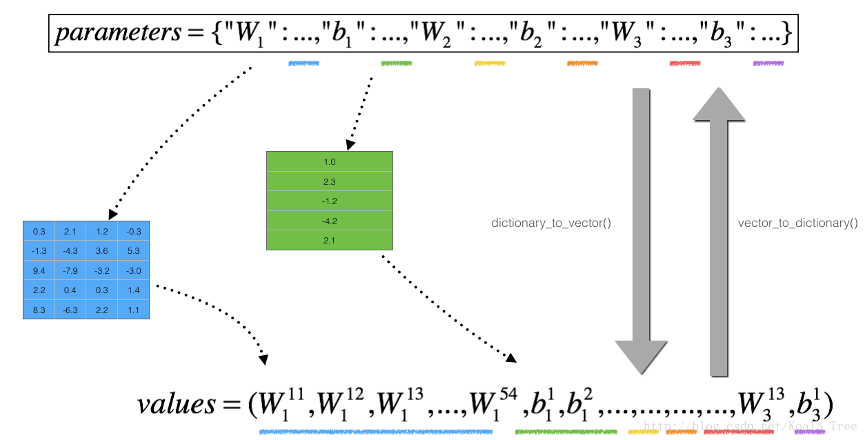
You will need these functions in gradient_check_n()

We have also converted the “gradients” dictionary into a vector “grad” using gradients_to_vector(). You don’t need to worry about that.

Exercise: Implement gradient_check_n().

Instructions: Here is pseudo-code that will help you implement the gradient check.

For each i in num_parameters:
- To compute J_plus[i]:
1. Set $\theta^{+}$ to np.copy(parameters_values)
2. Set $\theta^{+}_i$ to $\theta^{+}_i + \varepsilon$
3. Calculate $J^{+}_i$ using to forward_propagation_n(x, y, vector_to_dictionary( $\theta^{+}$ )).
- To compute J_minus[i]: do the same thing with $\theta^{-}$
- Compute $gradapprox[i] = \frac{J^{+}_i - J^{-}_i}{2 \varepsilon}$

Thus, you get a vector gradapprox, where gradapprox[i] is an approximation of the gradient with respect to parameter_values[i]. You can now compare this gradapprox vector to the gradients vector from backpropagation. Just like for the 1D case (Steps 1’, 2’, 3’), compute:

d i f f e r e n c e = ∥ g r a d - g r a d a p p r o x ∥ 2 ∥ g r a d ∥ 2 + ∥ g r a d a p p r o x ∥ 2 (3)

$difference = \frac {\| grad - gradapprox \|_2}{\| grad \|_2 + \| gradapprox \|_2 } \tag{3}$

# GRADED FUNCTION: gradient_check_n

def gradient_check_n(parameters, gradients, X, Y, epsilon = 1e-7):
    """
    Checks if backward_propagation_n computes correctly the gradient of the cost output by forward_propagation_n

    Arguments:
    parameters -- python dictionary containing your parameters "W1", "b1", "W2", "b2", "W3", "b3":
    grad -- output of backward_propagation_n, contains gradients of the cost with respect to the parameters. 
    x -- input datapoint, of shape (input size, 1)
    y -- true "label"
    epsilon -- tiny shift to the input to compute approximated gradient with formula(1)

    Returns:
    difference -- difference (2) between the approximated gradient and the backward propagation gradient
    """

    # Set-up variables
    parameters_values, _ = dictionary_to_vector(parameters)
    grad = gradients_to_vector(gradients)
    num_parameters = parameters_values.shape[0]
    J_plus = np.zeros((num_parameters, 1))
    J_minus = np.zeros((num_parameters, 1))
    gradapprox = np.zeros((num_parameters, 1))

    # Compute gradapprox
    for i in range(num_parameters):

        # Compute J_plus[i]. Inputs: "parameters_values, epsilon". Output = "J_plus[i]".
        # "_" is used because the function you have to outputs two parameters but we only care about the first one
        ### START CODE HERE ### (approx. 3 lines)
        thetaplus = np.copy(parameters_values)                                      # Step 1
        thetaplus[i][0] = thetaplus[i][0] + epsilon                                # Step 2
        J_plus[i], _ = forward_propagation_n(X, Y, vector_to_dictionary(thetaplus))                                  # Step 3
        ### END CODE HERE ###

        # Compute J_minus[i]. Inputs: "parameters_values, epsilon". Output = "J_minus[i]".
        ### START CODE HERE ### (approx. 3 lines)
        thetaminus = np.copy(parameters_values)                                     # Step 1
        thetaminus[i][0] = thetaminus[i][0] - epsilon                            # Step 2        
        J_minus[i], _ = forward_propagation_n(X, Y, vector_to_dictionary(thetaminus))                                  # Step 3
        ### END CODE HERE ###

        # Compute gradapprox[i]
        ### START CODE HERE ### (approx. 1 line)
        gradapprox[i] = (J_plus[i] - J_minus[i]) / (2.* epsilon)
        ### END CODE HERE ###

    # Compare gradapprox to backward propagation gradients by computing difference.
    ### START CODE HERE ### (approx. 1 line)
    numerator = np.linalg.norm(grad - gradapprox)                                           # Step 1'
    denominator = np.linalg.norm(grad) + np.linalg.norm(gradapprox)                                         # Step 2'
    difference = numerator / denominator                                          # Step 3'
    ### END CODE HERE ###

    if difference > 1e-7:
        print ("\033[93m" + "There is a mistake in the backward propagation! difference = " + str(difference) + "\033[0m")
    else:
        print ("\033[92m" + "Your backward propagation works perfectly fine! difference = " + str(difference) + "\033[0m")

    return difference

X, Y, parameters = gradient_check_n_test_case()

cost, cache = forward_propagation_n(X, Y, parameters)
gradients = backward_propagation_n(X, Y, cache)
difference = gradient_check_n(parameters, gradients, X, Y)

Your backward propagation works perfectly fine! difference = 0.285093156781

It seems that there were errors in the backward_propagation_n code we gave you! Good that you’ve implemented the gradient check. Go back to backward_propagation and try to find/correct the errors (Hint: check dW2 and db1). Rerun the gradient check when you think you’ve fixed it. Remember you’ll need to re-execute the cell defining backward_propagation_n() if you modify the code.

Can you get gradient check to declare your derivative computation correct? Even though this part of the assignment isn’t graded, we strongly urge you to try to find the bug and re-run gradient check until you’re convinced backprop is now correctly implemented.

Note
- Gradient Checking is slow! Approximating the gradient with $\frac{\partial J}{\partial \theta} \approx \frac{J(\theta + \varepsilon) - J(\theta - \varepsilon)}{2 \varepsilon}$ is computationally costly. For this reason, we don’t run gradient checking at every iteration during training. Just a few times to check if the gradient is correct.
- Gradient Checking, at least as we’ve presented it, doesn’t work with dropout. You would usually run the gradient check algorithm without dropout to make sure your backprop is correct, then add dropout.

Congrats, you can be confident that your deep learning model for fraud detection is working correctly! You can even use this to convince your CEO. :)

What you should remember from this notebook:
- Gradient checking verifies closeness between the gradients from backpropagation and the numerical approximation of the gradient (computed using forward propagation).
- Gradient checking is slow, so we don’t run it in every iteration of training. You would usually run it only to make sure your code is correct, then turn it off and use backprop for the actual learning process.

大树先生的博客

关注

18
点赞
踩
27

收藏

觉得还不错? 一键收藏
37
评论
吴恩达深度学习编程作业（2-1）- Initialization & Regularization & Gradient Checking

Part 1：Initialization、Part 2：Regularization、Part 3：Gradient Checking
复制链接

扫一扫