


python数据分析--- ch14-15 python计量回归模型
1.Ch14–python 回归分析
1.1 相关分析
1.1.1 相关系数的概念
r = ∑ ( x i − x ˉ ) ( y i − y ˉ ) ∑ ( x i − x ˉ ) 2 ∑ ( y i − y ˉ ) 2 r = \frac{\sum (x_i - \bar{x})(y_i - \bar{y})}{\sqrt{\sum (x_i - \bar{x})^2 \sum (y_i - \bar{y})^2}} r=∑(xi−xˉ)2∑(yi−yˉ)2∑(xi−xˉ)(yi−yˉ)
1.1.2 使用模拟数据计算变量之间的相关系数和绘图
# 导入包
import numpy as np
import statsmodels.tsa.stattools as sts
import matplotlib.pyplot as plt#绘图
import pandas as pd
import seaborn as sns#绘图
import statsmodels.api as sm
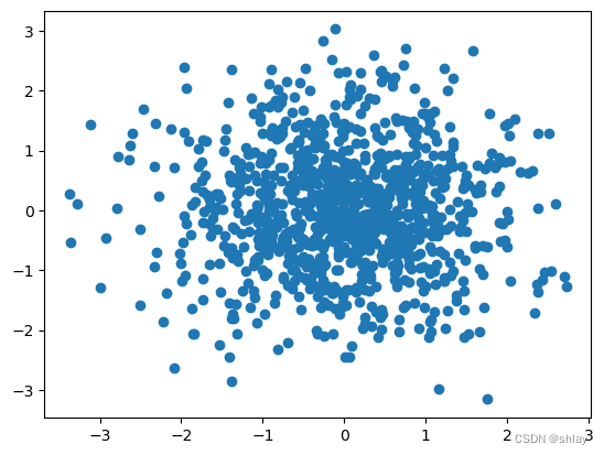
#生成随机数并绘制图形
X = np.random.randn(1000)
Y = np.random.randn(1000)
plt.scatter(X,Y)
plt.show()
print("correlation of X and Y is ")
np.corrcoef(X,Y)[0,1]
output
correlation of X and Y is
-0.0070692509611224395
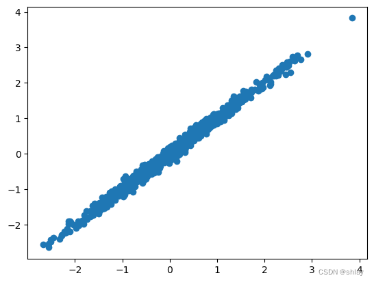
X = np.random.randn(1000)
Y = X + np.random.normal(0,0.1,1000)

plt.scatter(X,Y)
plt.show()
print("correlation of X and Y is ")
np.corrcoef(X,Y)[0,1]
output
correlation of X and Y is
0.9953589318626792
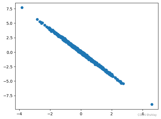
X = np.random.randn(1000)
Y = -2*X + np.random.normal(0,0.1,1000)
plt.scatter(X,Y)
plt.show()
print("correlation of X and Y is ")
np.corrcoef(X,Y)[0,1]
output
correlation of X and Y is
-0.9987776408463028
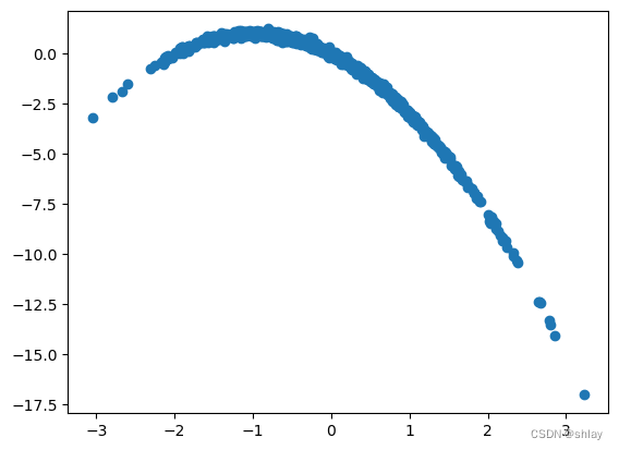
X = np.random.randn(1000)
Y = -X*X-2*X + np.random.normal(0,0.1,1000)
plt.scatter(X,Y)
plt.show()
print("correlation of X and Y is ")
np.corrcoef(X,Y)[0,1]
output
correlation of X and Y is
-0.8357355999573256
1.1.3 使用本地数据计算变量之间的相关系数和绘图
import pandas as pd
import numpy as np
import scipy.stats.stats as stats
r = ∑ ( x − m x ) ( y − m y ) ∑ ( x − m x ) 2 ∑ ( y − m y ) 2 r = \frac{\sum (x - m_x) (y - m_y)} {\sqrt{\sum (x - m_x)^2 \sum (y - m_y)^2}} r=∑(x−mx)2∑(y−my)2∑(x−mx)(y−my)
?stats.pearsonr
import numpy as np
from scipy import stats
x, y = [1, 2, 3, 4, 5, 6, 7], [10, 9, 2.5, 6, 4, 3, 2]
res = stats.pearsonr(x, y)
res
output
PearsonRResult(statistic=-0.8285038835884277, pvalue=0.021280260007523356)
数据文件“ch14_1.xls”下载
#读取数据并创建数据表,名称为data。
data=pd.DataFrame(pd.read_excel('./data/ch14_1.xls'))
#查看数据表前5行的内容
print(data.head())
#取adv和sale数据
x = np.array(data['adv'])
y = np.array(data['sale'])

r=stats.pearsonr(x,y)[0]
print(r)
output
time adv sale
0 1 35 50
1 2 50 100
2 3 56 120
3 4 68 180
4 5 70 175
0.9636816932556833
1.1.4 使用网上数据计算变量之间的相关系数和绘图
import pandas as pd
import numpy as np

# 创建一个包含10支股票的DataFrame
np.random.seed(42)  # 为了可重复性设置随机种子
stock_data = pd.DataFrame(np.random.randn(100, 10), columns=[f'Stock_{i}' for i in range(1, 11)])

# 将DataFrame转换为CSV文件
stock_data.to_csv('./data/ch14_2_stock_prices.csv', index=False)
print('CSV文件已生成。')
output
CSV文件已生成。
import pandas as pd
import seaborn as sns
import matplotlib.pyplot as plt
df = pd.read_csv('./data/ch14_2_stock_prices.csv')
df.head()
output
| Stock_1 | Stock_2 | Stock_3 | Stock_4 | Stock_5 | Stock_6 | Stock_7 | Stock_8 | Stock_9 | Stock_10 | |
|---|---|---|---|---|---|---|---|---|---|---|
| 0 | 0.496714 | -0.138264 | 0.647689 | 1.523030 | -0.234153 | -0.234137 | 1.579213 | 0.767435 | -0.469474 | 0.542560 |
| 1 | -0.463418 | -0.465730 | 0.241962 | -1.913280 | -1.724918 | -0.562288 | -1.012831 | 0.314247 | -0.908024 | -1.412304 |
| 2 | 1.465649 | -0.225776 | 0.067528 | -1.424748 | -0.544383 | 0.110923 | -1.150994 | 0.375698 | -0.600639 | -0.291694 |
| 3 | -0.601707 | 1.852278 | -0.013497 | -1.057711 | 0.822545 | -1.220844 | 0.208864 | -1.959670 | -1.328186 | 0.196861 |
| 4 | 0.738467 | 0.171368 | -0.115648 | -0.301104 | -1.478522 | -0.719844 | -0.460639 | 1.057122 | 0.343618 | -1.763040 |
correlation_matrix = df.corr()
plt.figure(figsize=(10, 8)) # 可以根据需要调整图形大小
sns.heatmap(correlation_matrix, annot=True, fmt=".2f", cmap='coolwarm', square=True)
plt.title('Heatmap of Stock Price Correlation')
plt.show()
output

1.2 一元回归分析
1.2.1 应用Python-statsmodels工具作一元线性回归分析
import pandas as pd
import numpy as np
import scipy.stats as ss
#读取数据并创建数据表,名称为data。
data=pd.DataFrame(pd.read_excel('./data/ch14_3.xls'))
print(data.head())
print(data.describe())
#此命令的含义是对销售额xse、人数rs等变量进行描述性统计分析。

#对数据进行相关分析
x = np.array(data['rs'])
y = np.array(data['xse'])

r=ss.pearsonr(x,y)[0]
#本命令的含义是对新产品销售额、销售人员人数等变量进行相关性分析
print ('相关系数为:',round(r,4))
print('相关系数矩阵为:\n', data.corr())
output
   dq  xse  rs
0   1  385  17
1   2  251  10
2   3  701  44
3   4  479  30
4   5  433  22
             dq         xse         rs
count  10.00000   10.000000  10.000000
mean    5.50000  446.600000  22.100000
std     3.02765  160.224287  12.705642
min     1.00000  217.000000   5.000000
25%     3.25000  362.500000  12.000000
50%     5.50000  422.000000  19.500000
75%     7.75000  555.500000  30.750000
max    10.00000  701.000000  44.000000
相关系数为: 0.9699
相关系数矩阵为:
            dq       xse        rs
dq   1.000000  0.218510  0.085207
xse  0.218510  1.000000  0.969906
rs   0.085207  0.969906  1.000000
# model matrix with intercept
X = sm.add_constant(x)
#least squares fit
model = sm.OLS(y, X)
fit = model.fit()
print(fit.summary())
output
                            OLS Regression Results
==============================================================================
Dep. Variable:                      y   R-squared:                       0.941
Model:                            OLS   Adj. R-squared:                  0.933
Method:                 Least Squares   F-statistic:                     126.9
Date:                Wed, 12 Jun 2024   Prob (F-statistic):           3.46e-06
Time:                        11:37:48   Log-Likelihood:                -50.301
No. Observations:                  10   AIC:                             104.6
Df Residuals:                       8   BIC:                             105.2
Df Model:                           1
Covariance Type:            nonrobust
==============================================================================
                 coef    std err          t      P>|t|      [0.025      0.975]
------------------------------------------------------------------------------
const        176.2952     27.327      6.451      0.000     113.279     239.311
x1            12.2310      1.086     11.267      0.000       9.728      14.734
==============================================================================
Omnibus:                        0.718   Durbin-Watson:                   1.407
Prob(Omnibus):                  0.698   Jarque-Bera (JB):                0.588
Skew:                          -0.198   Prob(JB):                        0.745
Kurtosis:                       1.879   Cond. No.                         52.6
==============================================================================
#画线性回归图
import matplotlib.pyplot as plt
plt.scatter(x, y)
plt.plot(x, fit.fittedvalues)

1.2.2 应用Python-sklearn工具作一元线性回归分析
import numpy as np
from sklearn import linear_model
import pandas as pd

# 假设data是已经定义并包含所需列的DataFrame
data=pd.DataFrame(pd.read_excel('./data/ch14_3.xls'))

# 确保data变量已经被定义且包含'rs'和'xse'列
x = np.array(data[['rs']])
y = np.array(data[['xse']])
x
output
array([[17],
[10],
[44],
[30],
[22],
[15],
[11],
[ 5],
[31],
[36]], dtype=int64)
data['rs']
output
0 17
1 10
2 44
3 30
4 22
5 15
6 11
7 5
8 31
9 36
Name: rs, dtype: int64
# 创建线性回归模型并拟合数据
clf = linear_model.LinearRegression()
clf.fit(x, y)

# 打印回归系数和截距
print("回归系数:", clf.coef_)
print("截距:", clf.intercept_)

# 计算并打印R²分数
r_squared = clf.score(x, y)
print("R-squared:", r_squared)

# 输入自变量值进行预测
# 假设你想预测'rs'为40时的'xse'值
prediction = clf.predict([[40]])
print("预测rs = 40时xse的值为 :", prediction[0])
output
回归系数: [[12.2309863]]
截距: [176.2952027]
R-squared: 0.9407180505879883
预测rs = 40时xse的值为 : [665.53465483]
1.3 多元线性回归数据分析
import pandas as pd
import numpy as np
import scipy.stats as ss
#读取数据并创建数据表,名称为data。
data=pd.DataFrame(pd.read_excel('./data/ch14_4.xls'))
print(data.head())
print(data.describe())
output
      TC  Q    PL    PF   PK
0  0.082  2  2.09  17.9  183
1  0.661  3  2.05  35.1  174
2  0.990  4  2.05  35.1  171
3  0.315  4  1.83  32.2  166
4  0.197  5  2.12  28.6  233
               TC             Q          PL          PF          PK
count  145.000000    145.000000  145.000000  145.000000  145.000000
mean    12.976097   2133.082759    1.972069   26.176552  174.496552
std     19.794577   2931.942131    0.236807    7.876071   18.209477
min      0.082000      2.000000    1.450000   10.300000  138.000000
25%      2.382000    279.000000    1.760000   21.300000  162.000000
50%      6.754000   1109.000000    2.040000   26.900000  170.000000
75%     14.132000   2507.000000    2.190000   32.200000  183.000000
max    139.422000  16719.000000    2.320000   42.800000  233.000000
#用数组对数据做相关分析
y= np.array(data['TC'])
x1= np.array(data['Q'])
x2= np.array(data['PL'])
x3= np.array(data['PF'])
x4= np.array(data['PK'])

r1=ss.pearsonr(x1,y)[0]
r2=ss.pearsonr(x2,y)[0]
r3=ss.pearsonr(x3,y)[0]
r4=ss.pearsonr(x4,y)[0]
print(f"r1={round(r1,4)};r2={round(r2,4)};r3={round(r3,4)};r4={round(r4,4)}")
output
r1=0.9525;r2=0.2513;r3=0.0339;r4=0.0272
#用数据框对数据做相关分析
corr_matrix = data.corr()
print('相关系数矩阵为:\n', data.corr())

plt.figure(figsize=(10, 8)) # 可以根据需要调整图形大小
sns.heatmap(corr_matrix, annot=True, fmt=".2f", cmap='coolwarm', square=True)
plt.title('Heatmap of data Correlation')
plt.show()
相关系数矩阵为:
           TC         Q        PL        PF        PK
TC  1.000000  0.952504  0.251338  0.033935  0.027202
Q   0.952504  1.000000  0.171450 -0.077349  0.002869
PL  0.251338  0.171450  1.000000  0.313703 -0.178145
PF  0.033935 -0.077349  0.313703  1.000000  0.125428
PK  0.027202  0.002869 -0.178145  0.125428  1.000000

1.3.1 多元回归分析的Python的statsmodels工具应用
import statsmodels.api as sm
from patsy import dmatrices
vars = ['TC','Q','PL','PF','PK']
df=data[vars]
#显示最后5条记录数据
print (df.tail())
output
          TC      Q    PL    PF   PK
140   44.894   9956  1.68  28.8  203
141   67.120  11477  2.24  26.5  151
142   73.050  11796  2.12  28.6  148
143  139.422  14359  2.31  33.5  212
144  119.939  16719  2.30  23.6  162
y,X=dmatrices('TC~Q+PL+PF+PK',data=data,return_type='dataframe')
print (y.head())
print (X.head())
model = sm.OLS(y, X)
fit = model.fit()
print (fit.summary())
output
      TC
0  0.082
1  0.661
2  0.990
3  0.315
4  0.197
   Intercept    Q    PL    PF     PK
0        1.0  2.0  2.09  17.9  183.0
1        1.0  3.0  2.05  35.1  174.0
2        1.0  4.0  2.05  35.1  171.0
3        1.0  4.0  1.83  32.2  166.0
4        1.0  5.0  2.12  28.6  233.0
                            OLS Regression Results
==============================================================================
Dep. Variable:                     TC   R-squared:                       0.923
Model:                            OLS   Adj. R-squared:                  0.921
Method:                 Least Squares   F-statistic:                     418.1
Date:                Wed, 12 Jun 2024   Prob (F-statistic):           9.26e-77
Time:                        11:38:18   Log-Likelihood:                -452.47
No. Observations:                 145   AIC:                             914.9
Df Residuals:                     140   BIC:                             929.8
Df Model:                           4
Covariance Type:            nonrobust
==============================================================================
                 coef    std err          t      P>|t|      [0.025      0.975]
------------------------------------------------------------------------------
Intercept    -22.2210      6.587     -3.373      0.001     -35.245      -9.197
Q              0.0064      0.000     39.258      0.000       0.006       0.007
PL             5.6552      2.176      2.598      0.010       1.352       9.958
PF             0.2078      0.064      3.242      0.001       0.081       0.335
PK             0.0284      0.027      1.073      0.285      -0.024       0.081
==============================================================================
Omnibus:                      135.057   Durbin-Watson:                   1.560
Prob(Omnibus):                  0.000   Jarque-Bera (JB):             4737.912
Skew:                           2.907   Prob(JB):                         0.00
Kurtosis:                      30.394   Cond. No.                     5.29e+04
==============================================================================
y,X=dmatrices('TC~Q+PL+PF',data=df,return_type='dataframe')
import statsmodels.api as sm
model = sm.OLS(y, X)
fit = model.fit()
print (fit.summary())
output
                            OLS Regression Results
==============================================================================
Dep. Variable:                     TC   R-squared:                       0.922
Model:                            OLS   Adj. R-squared:                  0.920
Method:                 Least Squares   F-statistic:                     556.5
Date:                Wed, 12 Jun 2024   Prob (F-statistic):           6.39e-78
Time:                        11:38:19   Log-Likelihood:                -453.06
No. Observations:                 145   AIC:                             914.1
Df Residuals:                     141   BIC:                             926.0
Df Model:                           3
Covariance Type:            nonrobust
==============================================================================
                 coef    std err          t      P>|t|      [0.025      0.975]
------------------------------------------------------------------------------
Intercept    -16.5443      3.928     -4.212      0.000     -24.309      -8.780
Q              0.0064      0.000     39.384      0.000       0.006       0.007
PL             5.0978      2.115      2.411      0.017       0.917       9.278
PF             0.2217      0.063      3.528      0.001       0.097       0.346
==============================================================================
Omnibus:                      142.387   Durbin-Watson:                   1.590
Prob(Omnibus):                  0.000   Jarque-Bera (JB):             5466.347
Skew:                           3.134   Prob(JB):                         0.00
Kurtosis:                      32.419   Cond. No.                     3.42e+04
==============================================================================
1.3.2 用scikit-learn工具作多元回归分析
import pandas as pd

print(data.shape)
print(data.head())
output
(145, 5)
      TC  Q    PL    PF   PK
0  0.082  2  2.09  17.9  183
1  0.661  3  2.05  35.1  174
2  0.990  4  2.05  35.1  171
3  0.315  4  1.83  32.2  166
4  0.197  5  2.12  28.6  233
feature_cols = ['Q', 'PL', 'PF', 'PK']
# use the list to select a subset of the original DataFrame
X = data[feature_cols]

# check the type and shape of X
print (type(X))
print (X.shape)

# select a Series from the DataFrame
y = data['TC']
# print the first 5 values
print (y.head())
output
<class 'pandas.core.frame.DataFrame'>
(145, 4)
0    0.082
1    0.661
2    0.990
3    0.315
4    0.197
Name: TC, dtype: float64
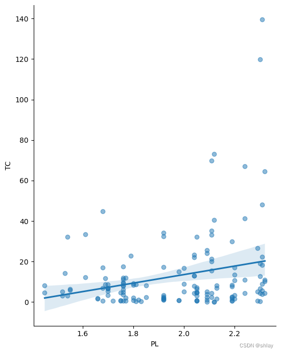
# import seaborn as sns   #seaborn程序包需要先安装
# #安装命令:pip install seaborn
# sns.pairplot(data, x_vars=['Q', 'PL', 'PF', 'PK'], y_vars='TC', height=7, aspect=0.8)

import seaborn as sns
import matplotlib.pyplot as plt

    # 使用lmplot绘制每个自变量与因变量之间的关系
for col in ['Q', 'PL', 'PF', 'PK']:
    sns.lmplot(x=col, y='TC', data=data, height=7, aspect=0.8, scatter_kws={'alpha':0.5})
plt.show()


1.4 线性回归模型
#构造训练集和测试集
from sklearn.model_selection import train_test_split
X_train, X_test, y_train, y_test = train_test_split(X, y, random_state=1)
# default split is 75% for training and 25% for testing
print(X_train.shape)
print(y_train.shape)
print(X_test.shape)
print(y_test.shape)

#线性回归分析的Scikit-learn工具应用
from sklearn.linear_model import LinearRegression
linreg = LinearRegression()
linreg.fit(X_train, y_train)
LinearRegression(copy_X=True, fit_intercept=True, n_jobs=1)
print(linreg.intercept_)
print(linreg.coef_)

# pair the feature names with the coefficients
zip(feature_cols, linreg.coef_)

#预测
y_pred = linreg.predict(X_test)
print(y_pred.round(decimals=4))
output
(108, 4)
(108,)
(37, 4)
(37,)
-15.546621299685215
[5.98807135e-03 5.68597073e+00 1.69334275e-01 9.00966074e-05]
[ 0.4819  4.1567  2.1491 32.6262  6.6678  1.4221  1.9241 17.8204  0.7097
  9.0636  4.1637  8.5665  5.6732  8.2366  3.96   25.3146 -0.9507  3.0294
  4.5084  2.7402 31.2073 12.9369  2.1043  3.8415 12.741  55.895  26.3795
 18.7322  6.7021  0.5052  1.4885 18.4282 13.5925 10.1431  2.7995  7.1969
 89.2625]
1.5 回归问题的评价测度
from sklearn import metrics
import numpy as np

# calculate MAE by hand
print("MAE by hand:",(10 + 0 + 20 + 10)/4)
# calculate MAE using scikit-learn
print ("MAE:",metrics.mean_absolute_error(y_test, y_pred))

# calculate MSE by hand
print ("MSE by hand:",(10**2 + 0**2 + 20**2 + 10**2)/4.)
# calculate MSE using scikit-learn
print ("MSE:",metrics.mean_squared_error(y_test, y_pred))

# calculate RMSE by hand
print ("RMSE by hand:",np.sqrt((10**2 + 0**2 + 20**2 + 10**2)/4.))
# calculate RMSE using scikit-learn
print ("RMSE:",np.sqrt(metrics.mean_squared_error(y_test, y_pred)))
output
MAE by hand: 10.0
MAE: 3.559135213796553
MSE by hand: 150.0
MSE: 77.98080985164937
RMSE by hand: 12.24744871391589
RMSE: 8.830674371283846
2. Ch15–python 时间序列分析
2.1 准备工作
2.1.1 加载包
# 加载包
import warnings
warnings.filterwarnings('ignore')
import pandas as pd
import numpy as np
import matplotlib.pyplot as plt
import statsmodels.api as sm
from statsmodels.tsa.arima.model import ARIMA
from sklearn.metrics import mean_squared_error, mean_absolute_error
from datetime import datetime

#全局配置
#中文字符设定 plt.rcParams属性总结
plt.rcParams['font.sans-serif']=['SimHei']
plt.rcParams['axes.unicode_minus']=False
2.1.2 数据读取及预处理
数据文件“csh601318_processed.csv”下载
df = pd.read_csv('./data/sh601318_processed.csv',index_col='Date')
df.head()
output
| Close | |
|---|---|
| Date | |
| 2015-01-05 | 76.16 |
| 2015-01-06 | 73.73 |
| 2015-01-07 | 73.41 |
| 2015-01-08 | 71.08 |
| 2015-01-09 | 72.84 |
#读取已处理好的数据

df_601318 = df[['Close']]
df_601318.index = pd.to_datetime(df_601318.index, format='%Y-%m-%d') # 将Date列转换为datetime格式
# 查看数据的基本信息
print(df_601318.head())
output
            Close
Date
2015-01-05  76.16
2015-01-06  73.73
2015-01-07  73.41
2015-01-08  71.08
2015-01-09  72.84
print(df_601318.info())
output
<class 'pandas.core.frame.DataFrame'>
DatetimeIndex: 2033 entries, 2015-01-05 to 2023-05-15
Data columns (total 1 columns):
 #   Column  Non-Null Count  Dtype
---  ------  --------------  -----
 0   Close   2033 non-null   float64
dtypes: float64(1)
memory usage: 31.8 KB
None
print(df_601318.describe())
output
             Close
count  2033.000000
mean     59.039838
std      18.942363
min      25.110000
25%      42.840000
50%      58.380000
75%      76.520000
max      93.380000
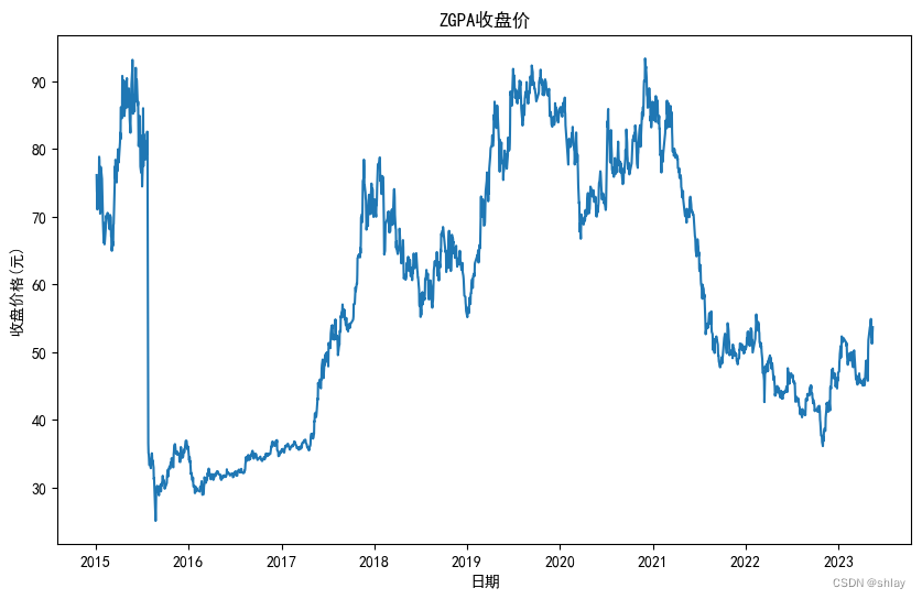
2.2 可视化股票价格
#对数据进行可视化,以了解股票价格的趋势和变化。
plt.figure(figsize=(10, 6))
plt.plot(df_601318['Close'])
plt.title('ZGPA收盘价')
plt.xlabel('日期')
plt.ylabel('收盘价格(元)')
plt.show()
2.3 单位根检验
# 进行ADF检验
result = sm.tsa.stattools.adfuller(df_601318['Close'])
print('ADF Statistic: %f' % result[0])
print('p-value: %f' % result[1])
print('Critical Values:')
for key, value in result[4].items():
    print('\t%s: %.3f' % (key, value))
output
ADF Statistic: -1.894778
p-value: 0.334522
Critical Values:
	1%: -3.434
	5%: -2.863
	10%: -2.568
无法拒绝原假设,认为数据是非平稳的。
2.4 差分
2.4.1 一阶差分
# 进行一阶差分
diff1 = df_601318['Close'].diff().dropna()
2.4.2 一阶差分ADF检验
# 进行ADF检验
result = sm.tsa.stattools.adfuller(diff1)
print('ADF Statistic: %f' % result[0])
print('p-value: %f' % result[1])
print('Critical Values:')
for key, value in result[4].items():
    print('\t%s: %.3f' % (key, value))
output
ADF Statistic: -8.640510
p-value: 0.000000
Critical Values:
	1%: -3.434
	5%: -2.863
	10%: -2.568
一阶差分后序列平稳
2.4.3 绘制一阶差分后的时序图
# 绘制差分后的时间序列图
fig, ax = plt.subplots(2, 1, figsize=(8, 12))
ax[0].plot(df_601318.index, df_601318['Close'])
ax[0].set_title('原始数据')
ax[1].plot(diff1.index, diff1)
ax[1].set_title('一阶差分')
# ax[2].plot(diff2.index, diff2)
# ax[2].set_title('二阶差分')
plt.show()

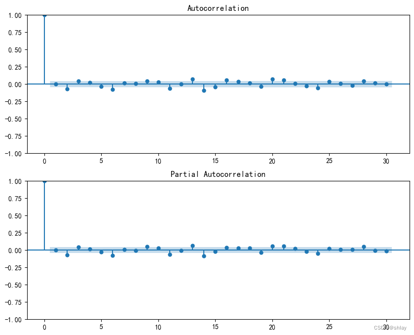
2.5 绘制自相关图和偏自相关图
2.5.1 绘制原序列自相关图和偏自相关图
# 绘制自相关图和偏自相关图
fig, axes = plt.subplots(2, 1, figsize=(10,8))
sm.graphics.tsa.plot_acf(df_601318['Close'], lags=50, ax=axes[0])
sm.graphics.tsa.plot_pacf(df_601318['Close'], lags=30, ax=axes[1])
plt.show()

2.5.2 绘制一阶差分后自相关图和偏自相关图
# 绘制自相关图和偏自相关图
fig, axes = plt.subplots(2, 1, figsize=(10,8))
sm.graphics.tsa.plot_acf(diff1, lags=30, ax=axes[0])
sm.graphics.tsa.plot_pacf(diff1, lags=30, ax=axes[1])
plt.show()
2.6 划分训练集和测试集
2.6.1 按照指定的百分比划分,如:8:2,7:3等
# 假设df是处理好的股票数据
train_size = int(len(df_601318) * 0.8)
train_df = df_601318[:train_size]
test_df = df_601318[train_size:]
# 输出训练集和测试集的数据量
print("训练集数据量:", len(train_df))
print("测试集数据量:", len(test_df))
output
训练集数据量: 1626
测试集数据量: 407
2.6.2 按照指定的日期划分,如:2022-12-31
# 假设df是处理好的股票数据
split_date = datetime(2021, 12, 31)
train_df = df_601318[df_601318.index <= split_date]
test_df = df_601318[df_601318.index > split_date]

# 输出训练集和测试集的数据量
print("训练集数据量:", len(train_df))
print("测试集数据量:", len(test_df))
output
训练集数据量: 1705
测试集数据量: 328
test_df.head()
output
| Close | |
|---|---|
| Date | |
| 2022-01-04 | 51.00 |
| 2022-01-05 | 52.07 |
| 2022-01-06 | 51.30 |
| 2022-01-07 | 52.94 |
| 2022-01-10 | 53.08 |
2.7 模型拟合
我们可以使用 ARIMA 函数来拟合 ARIMA 模型并进行预测。首先,需要确定 ARIMA 模型的参数。可以通过观察 ACF 和 PACF 图来初步选择参数。在这里,我们将选择 ARIMA(1,1,1) 模型。
# 拟合ARIMA(1,1,1)模型并预测训练集数据
model = ARIMA(train_df, order=(1, 1, 1))
model_fit = model.fit()
# 模型概述
print(model_fit.summary())
output
                               SARIMAX Results
==============================================================================
Dep. Variable:                  Close   No. Observations:                 1705
Model:                 ARIMA(1, 1, 1)   Log Likelihood               -3295.505
Date:                Wed, 12 Jun 2024   AIC                           6597.010
Time:                        11:41:15   BIC                           6613.333
Sample:                             0   HQIC                          6603.052
                               - 1705
Covariance Type:                  opg
==============================================================================
                 coef    std err          z      P>|z|      [0.025      0.975]
------------------------------------------------------------------------------
ar.L1         -0.7986      0.117     -6.807      0.000      -1.029      -0.569
ma.L1          0.8396      0.105      8.020      0.000       0.634       1.045
sigma2         2.8013      0.017    160.271      0.000       2.767       2.836
===================================================================================
Ljung-Box (L1) (Q):                   2.02   Jarque-Bera (JB):           5344375.75
Prob(Q):                              0.16   Prob(JB):                         0.00
Heteroskedasticity (H):               0.29   Skew:                           -10.32
Prob(H) (two-sided):                  0.00   Kurtosis:                       276.58
===================================================================================

Warnings:
[1] Covariance matrix calculated using the outer product of gradients (complex-step).
train_pred = model_fit.predict(typ='levels')

# 预测测试集数据
test_pred = model_fit.forecast(steps=len(test_df))

# 输出训练集和测试集的预测数据
print("训练集预测数据:\n", train_pred)
print("测试集预测数据:\n", test_pred)
output
训练集预测数据:
 Date
2015-01-05     0.000000
2015-01-06    76.160008
2015-01-07    73.639795
2015-01-08    73.473245
2015-01-09    70.935963
                ...
2021-12-27    49.766963
2021-12-28    50.031091
2021-12-29    50.863590
2021-12-30    50.812922
2021-12-31    50.391148
Name: predicted_mean, Length: 1705, dtype: float64
测试集预测数据:
 1705    50.425828
1706    50.413187
1707    50.423283
1708    50.415220
1709    50.421659
          ...
2028    50.418800
2029    50.418800
2030    50.418800
2031    50.418800
2032    50.418800
Name: predicted_mean, Length: 328, dtype: float64
# 可视化训练集和测试集的实际数据和预测数据
plt.figure(figsize=(12,6))
plt.plot(train_df.index, train_df.values, label='训练数据')
plt.plot(train_df.index, train_pred.values, label='训练数据预测值')
plt.plot(test_df.index, test_df.values, label='测试数据')
plt.plot(test_df.index, test_pred.values, label='测试数据预测值')
plt.legend()
plt.title('ARIMA(1,1,1)模型拟合结果')
plt.xlabel('日期')
plt.ylabel('收盘价格')
plt.show()
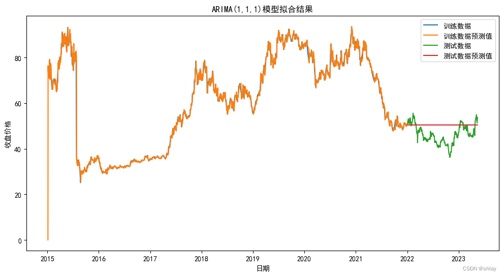
思考:ARIMA在训练集上拟合的比较好,但在测试集上,所有的预测值几乎都相等,为什么?问题出在哪?怎么解决?
2.8 模型评价
2.8.1 计算评估指标
为了评估模型的预测效果,我们需要计算一些常用的评估指标,包括均方误差(Mean Squared Error,MSE)、均方根误差(Root Mean Squared Error,RMSE)、平均绝对误差(Mean Absolute Error,MAE)和平均绝对百分误差(Mean Absolute Percentage Error,MAPE)等。
这些指标的计算公式如下:
M S E = 1 n ∑ i = 1 n ( y i − y ^ i ) 2 MSE = \frac{1}{n} \sum_{i=1}^{n}(y_i - \hat{y}_i)^2 MSE=n1i=1∑n(yi−y^i)2
R M S E = M S E RMSE = \sqrt{MSE} RMSE=MSE
M A E = 1 n ∑ i = 1 n ∣ y i − y ^ i ∣ MAE = \frac{1}{n} \sum_{i=1}^{n}|y_i - \hat{y}_i| MAE=n1i=1∑n∣yi−y^i∣
M A P E = 1 n ∑ i = 1 n ∣ y _ i − y ^ i y i ∣ × 100 MAPE = \frac{1}{n} \sum_{i=1}^{n}|\frac{y\_i - \hat{y}_i}{y_i}| \times 100% MAPE=n1i=1∑n∣yiy_i−y^i∣×100
其中, y i y_i yi 表示真实值, y ^ i \hat{y}_i y^i 表示预测值, n n n 表示样本数量。
代码如下:
# 计算评估指标
mse = mean_squared_error(test_df.values, test_pred.values)
rmse = np.sqrt(mse)
mae = mean_absolute_error(test_df.values, test_pred.values)
mape = np.mean(np.abs((test_df.values - test_pred.values) / test_df.values)) * 100

# 打印评估指标
print('MSE: %.2f' % mse)
print('RMSE: %.2f' % rmse)
print('MAE: %.2f' % mae)
print('MAPE: %.2f%%' % mape)
output
MSE: 33.86
RMSE: 5.82
MAE: 4.92
MAPE: 11.28%
- 接下来,我们可以
绘制模型的残差图(Residual Plot),来评估模型是否存在系统性误差。如果模型的残差是随机的、没有规律性,那么说明模型拟合得比较好;如果残差呈现出一定的规律性,那么说明模型还存在一些问题。
2.8.2 残差检验
(1) 绘制残差图
# 计算训练集和测试集的残差
train_resid = train_df['Close'] - train_pred.values
test_resid = test_df['Close'] - test_pred.values

# 绘制训练集和测试集的残差图
plt.figure(figsize=(12,10))
plt.subplot(211)
plt.plot(train_resid)
plt.title('训练数据残差图')
plt.xlabel('年份')
plt.ylabel('残差')

plt.subplot(212)
plt.plot(test_resid)
plt.title('测试数据残差图')
plt.xlabel('年份')
plt.ylabel('残差')
plt.show()

(2) 对残差进行平稳性检验
# 对训练集残差进行平稳性检验
result3 = sm.tsa.stattools.adfuller(train_resid)
print('训练集残差ADF检验结果:')
print('ADF Statistic: %f' % result3[0])
print('p-value: %f' % result3[1])
print('Critical Values:')
for key, value in result3[4].items():
    print('\t%s: %.3f' % (key, value))

# 对测试集残差进行平稳性检验
result4 = sm.tsa.stattools.adfuller(test_resid)
print("")
print('测试集残差ADF检验结果:')
print('ADF Statistic: %f' % result4[0])
print('p-value: %f' % result4[1])
print('Critical Values:')
for key, value in result4[4].items():
    print('\t%s: %.3f' % (key, value))
output
训练集残差ADF检验结果:
ADF Statistic: -7.788862
p-value: 0.000000
Critical Values:
	1%: -3.434
	5%: -2.863
	10%: -2.568

测试集残差ADF检验结果:
ADF Statistic: -1.734568
p-value: 0.413396
Critical Values:
	1%: -3.451
	5%: -2.870
	10%: -2.572
根据结果,训练集残差ADF 统计量为-8.386454,远小于 1% 的临界值-3.616,因此我们可以拒绝原假设(序列具有单位根非平稳性),接受备择假设,即序列是平稳的。 P 值为 0,说明序列的单位根非常显著地低于 5% 的显著性水平,进一步支持序列的平稳性。
2.9 小结
对某股票的历史股价数据进行时序分析和预测,具体步骤如下:
-
1.首先加载相应的包
-
2.数据的读取和初步探索
-
3.平稳性检验
-
4.确定差分阶数
-
5.通过自相关图和偏自相关图来确定拟合模型
-
6.拟合ARIMA模型并进行预测
-
7.对预测结果进行评估
本次分析表明,ARIMA模型可以用于股票价格的预测。但是,在实际应用中需要注意,股票价格受到多种因素的影响,仅使用历史价格数据进行预测是不够准确的,需要考虑其他因素的影响。此外,ARIMA模型的预测精度也会受到模型参数的选择和数据质量的影响,需要进行不断的调整和优化。


 被折叠的 条评论
为什么被折叠?
被折叠的 条评论
为什么被折叠?
 到【灌水乐园】发言


