ex3_3 Equality constrains and unrestricted variables

matlab source code:

% Ex3_3.m
% Example 3.3
%  Optimization Using MATLAB by P.Venkataraman
%
%	Using drawLine.m 
%
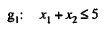
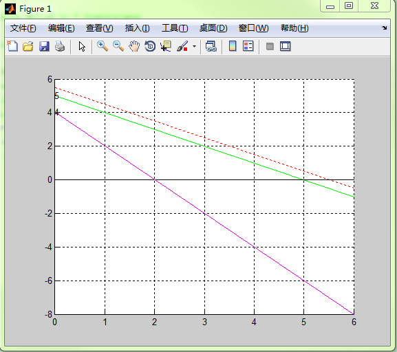
drawLine(0,6,1,1,5,'l');
drawLine(0,6,2,1,4,'e');
drawLine(0,6,1,1,1,'g');
drawLine(0,6,2,-1,8,'n');
xlabel('Hours spent studying');
ylabel('Hours of pin ball');
title('Example 3.3 -Equality Constraint and Negative Design Variables')
grid

% drawLine.m
% Drawing linear constraints for LP programming problems
% Dr. P.Venkataraman
% Optimization Using Matlab
% Chapter 3 - linear Programming
%
% Lines are represented as: ax + by = c ( c >= 0)
% x1, x2 indicate the range of x for the line
% typ indicates type of line being drawn l (<=)
%                                        g, (>=)
%                                        n  (none)
%
% The function will draw line(s) in the figure window
% the green line represents the actual value 
% of the constraint
% the red dashed line is 10 % larger or smaller
% (in lieu of hash marks)
% the limit constraints are identifies in magenta color
% the objective function is in blue dashed lines
%
function ret = drawLine(x1,x2,a,b,c,typ)

% recognize the types and set color
if (typ == 'n') 
   str1 = 'b';
   str2 = 'b';
   cmult = 1;
elseif (typ == 'e')
      str1 ='m';
      str2 ='m';
 else
   str1 = 'g';
   str2 = 'r';
end

% values for drawing hash marks
% depending on the direction of inequality
if (typ ~= 'n' | 'e') 
   if (typ == 'l')
      cmult = +1;
   else cmult = -1;
   end
end

% set up a factor for drawing the hash constraint
if (abs(c) >= 10)
   cfac = 0.025;
elseif (abs(c)> 5) & (abs(c) <  10)
   cfac = 0.05;
else
   cfac = 0.1;
end

if (c == 0 ) 
   cdum = cmult*0.1; 
else
   cdum = (1 + cmult* cfac)*c;
end

% if b = 0 then determine end points of line x line
if ( b ~= 0)
   y1 = (c - a*x1)/b;
   y1n = (cdum - a* x1)/b;
   y2 = (c - a* x2)/b;
   y2n = (cdum - a*x2)/b;
else
   % identfy limit constraints by magenta color
   str1 = 'm';
   str2 = 'm';
   y1 = x1; % set  y1 same length as input x1
   y2 = x2;  % set y2 same length as input x2
   x1 = c/a;  % adjust x1 to actual value
   x2 = c/a;  % adjust x2 to actual value
   y1n = 0;  % set y = 0;
   y2n = 0;  % set  y = 0
end

if (a == 0) 
   str1 = 'm'; % set color for limit line
   str2 = 'm'; % set color for limit line
end;
% draw axis with solid black color

hh = line([x1,x2],[0,0]);
set(hh,'LineWidth',1,'Color','k');

hv = line([0,0],[x1,x2]);
set(hv,'LineWidth',1,'Color','k');

% start drawing the lines

h1 = line([x1 x2], [y1,y2]);

if (typ == 'n') 
   set(h1,'LineWidth',2,'LineStyle','--','Color',str1);
else
   set(h1,'LineWidth',1,'LineStyle','-','Color',str1);
end

if (b ~= 0)&(a ~= 0)
   text(x1,y1,num2str(c));
end
if( b == 0)|(a == 0)| (typ == 'n') | (typ == 'e')
   grid
   ret = [h1];
   return, end 
grid;
h2 = line([x1 x2], [y1n,y2n]);
set(h2,'LineWidth',0.5,'LineStyle',':','Color',str2);
grid
hold on
ret = [h1 h2];

here, I would like to analysis drawLine.m

% drawLine.m
% Drawing linear constraints for LP programming problems
% Dr. P.Venkataraman
% Optimization Using Matlab
% Chapter 3 - linear Programming
%
% Lines are represented as: ax + by = c ( c >= 0)
% x1, x2 indicate the range of x for the line
% typ indicates type of line being drawn l (<=)
%                                        g, (>=)
%                                        n  (none)
%
% The function will draw line(s) in the figure window
% the green line represents the actual value 
% of the constraint
% the red dashed line is 10 % larger or smaller
% (in lieu of hash marks)
% the limit constraints are identifies in magenta color
% the objective function is in blue dashed lines
%
function ret = drawLine(x1,x2,a,b,c,typ)


% recognize the types and set color
if (typ == 'n') 
   str1 = 'b';
   str2 = 'b';
   cmult = 1;
elseif (typ == 'e')
      str1 ='m';
      str2 ='m';
 else
   str1 = 'g';
   str2 = 'r';
end

str1是第一根线的颜色,str2是第二根线的颜色


% values for drawing hash marks
% depending on the direction of inequality
if (typ ~= 'n' | 'e') 
   if (typ == 'l')
      cmult = +1;
   else cmult = -1;
   end
end
确定第二根线的挪动方向

% set up a factor for drawing the hash constraint
if (abs(c) >= 10)
   cfac = 0.025;
elseif (abs(c)> 5) & (abs(c) <  10)
   cfac = 0.05;
else
   cfac = 0.1;
end


if (c == 0 ) 
   cdum = cmult*0.1; 
else
   cdum = (1 + cmult* cfac)*c;
end
确定挪动的距离

% if b = 0 then determine end points of line x line
if ( b ~= 0)
   y1 = (c - a*x1)/b;
   y1n = (cdum - a* x1)/b;
   y2 = (c - a* x2)/b;
   y2n = (cdum - a*x2)/b;

确定第一根线和第二根线的方程

h1 = line([x1 x2], [y1,y2]);  [x1 x2]为x的范围, [y1,y2]为y的范围

h2 = line([x1 x2], [y1n,y2n]);
else
   % identfy limit constraints by magenta color
   str1 = 'm';
   str2 = 'm';
   y1 = x1; % set  y1 same length as input x1
   y2 = x2;  % set y2 same length as input x2
   x1 = c/a;  % adjust x1 to actual value
   x2 = c/a;  % adjust x2 to actual value
   y1n = 0;  % set y = 0;
   y2n = 0;  % set  y = 0

当线垂直的情况
end


if (a == 0) 
   str1 = 'm'; % set color for limit line
   str2 = 'm'; % set color for limit line
end;
% draw axis with solid black color


hh = line([x1,x2],[0,0]);
set(hh,'LineWidth',1,'Color','k');


hv = line([0,0],[x1,x2]);
set(hv,'LineWidth',1,'Color','k');


% start drawing the lines


h1 = line([x1 x2], [y1,y2]);


if (typ == 'n') 
   set(h1,'LineWidth',2,'LineStyle','--','Color',str1);
else
   set(h1,'LineWidth',1,'LineStyle','-','Color',str1);
end


if (b ~= 0)&(a ~= 0)
   text(x1,y1,num2str(c));
end
if( b == 0)|(a == 0)| (typ == 'n') | (typ == 'e')
   grid
   ret = [h1];
   return, end 
grid;
h2 = line([x1 x2], [y1n,y2n]);
set(h2,'LineWidth',0.5,'LineStyle',':','Color',str2);
grid
hold on
ret = [h1 h2];

% Ex3_3.m
% Example 3.3
%  Optimization Using MATLAB by P.Venkataraman
%
% Using drawLine.m 
%
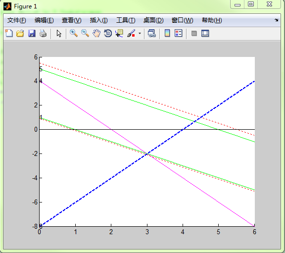
drawLine(0,6,1,1,5,'l');

第一条线

画了过后

第一根线是绿线, 第二根线是红线, 表示绿线的左下部分是可行区域

drawLine(0,6,2,1,4,'e');

第二条线

画了过后, 这里用紫线表示

drawLine(0,6,1,1,1,'g');

第三条线

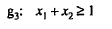
画了过后

红线在此绿线的左下角,则说明可行区域在绿线的右上角部分

drawLine(0,6,2,-1,8,'n');

目标函数

画完过后,这里用蓝虚线表示,这里目标函数的意义为与Y轴截距的负值

xlabel('Hours spent studying');
ylabel('Hours of pin ball');
title('Example 3.3 -Equality Constraint and Negative Design Variables')
grid